Download
1 / 27
340 likes | 708 Views
CT Principle. Preprocessing. Blockdiagram image processor. Blockdiagram image processor. An image processor consists on 4 functional blocks: 1: Pre- processor 2. Convolver 3. Backprojector 4. Imager

E N D
CT Principle Preprocessing
Blockdiagram image processor An image processor consists on 4 functional blocks: 1: Pre- processor 2. Convolver 3. Backprojector 4. Imager The data measurement system supplies the scan data in serial order to the receiver module, which is a part of the pre- processor.
Blockdiagram pre- processor • A pre- processor has to compensate the measured data for : • Electrical drifts • Dose variations • X-ray attenuation law • Beam hardening • Mechanical deviations of the scanning system • The input (measured data from the aquisition system) is called a reading, the output a projection.
PGA decoding The signals from the detector have a very wide range. To cover the whole dynamic range of input signals, a „ProgrammableGain Amplifier“ (PGA) is used (also called FPA, floating point amplifier). PGA: The PPA is an amplifier which selects its gain automatically. The selected gain can be 1, 8 or 64. The gain used is indicated by the two bits called `PGA Bits´. PGA Decoding:In order to calculate the actual attenuation, the PGA bits are decoded in the SMI. This is done in the preprocessing step „PGA decoding“ (also called „FPA decoding“).
PGA decoding Amplification 64:If the signal from the detector was very small (i.e., high absorption in the scanfield), the amplifier will have used a factor of 64. The resulting data in the SMI will be the 14 bit from the ADC, preceeded by many zeroes, in other words, a rather small numerical value. Amplification 8:If the amplification was 8, the signal was larger. In the SMI, the 14 bit are shifted 3 bit to the left, equaling a multiplication by 8, or a larger numerical value. Amplifiaction 1: If the signal from the detector was large (e.g., only air in the scanfield), the PGA will have used an amplification of 1. This will result in a large number in the SMI, because the 14 bit are shifted 6 bit to the left, equaling a multiplication by 64 or a rather large numerical value.
Offset correction Offset voltage : In the DMS, ADCs are used that can´t measure negative voltages. This would falsify the measurement, if very small detector signals ( = high absorptions ) have to be measured. To avoid this, in the DMS an offset voltage is added to the signal, the signal is measured, and in the SMI the offset signal subtracted again, leaving the true value only. Offsets are channel specific: Because the analogue offset may be slightly different for each ADC, or, to be precise, even for every integrator board channel, the actual offset has to be measured prior to the scan for every channel. Offset measurement: With each scan start, a measurement is started without X-ray and the data are stored in the image processor as offset data.
Logarithmation Logarithmation is done because the attenuation of an X-ray beam follows an exponential law. I = Io e - µ d The calculation of the object attenuation „A“ requires the calculation of the logarithmic value of the measured radiation intensities I and I 0: A= ln I 0 – ln I The logarithmation is done using a table of log values.
Normalization During the measurement, the intensity Io of the X-ray beam varies (exaggerated in the picture for clear visualization). Monitor value: A monitor element measures the unattenuated radiation as a reference value.This value is called “Monitor value”. Normalization : During the preprocessing step “Normalization” , this monitor value IM is substracted from each channel value I: In 1/I– In 1/IM
Calibration Each detector has a different sensitivity. This can vary with the time and must be compensated. The channel specific sensitivity differences are compensated by calibration. Technically, that means taking an air scan and then subtracting the channel values obtained in air from the normalized channel values. Then pre- processing step calibration requires the base calibration tables, that are measured during the last calibration. During the last tune up, the differences of each combination of kV, mA, slice width etc. were measured, so that only the base calibration is required on a daily basis. The other calibration tables for different settings of kV, mA etc are calculated from the difference tables and the base calibration table.
Channel Correction • Technically, the pre- processing step „channel correction“ is a multiplication of each channel value with a correction factor. • Because a correction is needed for many reasons, several individual tune- up tables contribute to the resulting one factor in the pre- processing. • Channel correction includes: • Beam hardening correction • Cosine correction • Channel coefficient correction and • Water scaling
Beam – Hardening Correction X-ray spectrum: Tubes generate polychromatic radiation, i.e.different wavelength are contained in the spectrum. Just as with visible light, the higher energies or shorter wavelength can penetrate the objects better than the softer part of the spectrum. Beam hardening causes in homogenous objects (e.g. a water phantom) an inhomogeneity. That means, the CT values in the center are different from the outer values. The correction is done by taking data of a reference phantom (mostly a 20cm water phantom) and the correction data are used during pre- processing step „beam hardening“ for the correction of the scan data.
Cosine - Correction Measured attenuation: The Cosine – Correction considers that the x-ray beam is fan shaped. The length of the path of the radiation through an object depends on the angle alpha between the central beam and any other beam. Corrected attenuation: The correction of the different channel outputs is done by using the cosine function. For each channel, the table contains the cosine-value of the corresponding fan angle „alpha“. The measured attenuation is multiplied with the table values.
Channel Coefficient Correction Just like „Calibration“, the pre-processing step ´Channel Correction´ compensates for sensitivity differences of the detector. The difference is that the Channel correction compensates for nonlinearities in the area of attenuated radiation, i.e., with an object is in the scan field. Parameter: The parameters which determine the detected radiation energy are: Tube Voltage Slice Thickness Object Attenuation (Head or body) Correction tables: The sensitivity compensation is done with values which are determined during the tune-up.
Water Scaling The water scaling sets CT value of water to 0 HU. This factor depends on the energy received by the detector; the parameters for the scaling are: - tube voltage - tube current - slice thickness