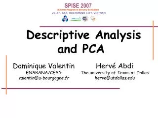
Descriptive Analysis and PCA
310 likes | 486 Views
Descriptive Analysis and PCA. Dominique Valentin ENSBANA/CESG valentin@u-bourgogne.fr. Hervé Abdi The university of Texas at Dallas herve@utdallas.edu. Back to the yogurt example. Texture Thickness: consistency of the mass in the mouth

Descriptive Analysis and PCA
E N D
Presentation Transcript
Descriptive Analysis and PCA Dominique Valentin ENSBANA/CESG valentin@u-bourgogne.fr Hervé Abdi The university of Texas at Dallas herve@utdallas.edu
Back to the yogurt example Texture Thickness: consistency of the mass in the mouth Rate of Melt:amount of product melted after a certain pressure of the tongue Graininess: amount of particle in mass Mouth coating: amount of film left on the mouth surfaces Basic tastes Sweet: Sucrose Sour:lactic acid Bitter: caffeine Salty:sodium chloride Arôme Water: taste like water down Flour: 1 spoon of flavor mixed in water Wood: cutting from pencil sharpening Chalk: smecta Milk: whole milk Raw pie crust: commercial raw pie crust Cream: crème fraiche Hazelnut: : hazelnut powder earthy: earth Mushroom: dry mushrooms soaked in water
Back to the yogurt example 9 panélistes 5 yogurts: 2 cow milk yogurts 3 soy yogurts Amer Pas du tout Très Salé Pas du tout Très Astringent Pas du tout
Back to the yogurt example Épais – thickness Farineux - Flour 10,00 10,00 a 8,00 8,00 ab ab a bc bc ab 6,00 6,00 d Intensité moyenne Intensité moyenne 4,00 b b 4,00 2,00 2,00 0,00 0,00 soja sojasun sojade velouté leaderprice soja sojasun sojade velouté carrefour danone carrefour danone Gras – Mouth coating Fondant - melt 10,00 a ab 8,00 10,00 ab ab ab 6,00 b abc 8,00 abc abc Intensité moyenne 4,00 c 6,00 Intensité moyenne 2,00 4,00 0,00 2,00 soja sojasun sojade velouté leaderprice 0,00 carrefour danone soja sojasun sojade velouté leaderprice carrefour danone Texture leaderprice
Back to the yogurt example Sucré - Sweet Acide - Sour a 10,00 10,00 8,00 8,00 ab ab ab bc ab cd ab 6,00 6,00 cd cd Intensité moyenne Intensité moyenne 4,00 4,00 2,00 2,00 0,00 0,00 soja sojasun sojade velouté leaderprice soja sojasun sojade velouté carrefour danone carrefour danone Amer - Bitter 10,00 8,00 a 6,00 a a a a Intensité moyenne 4,00 2,00 0,00 soja sojasun sojade velouté leaderprice carrefour danone Taste leaderprice astringent 10,00 a abc 8,00 abc abc 6,00 c Intensité moyenne 4,00 2,00 0,00 soja sojasun sojade velouté leaderprice carrefour danone
Back to the yogurt example Noisette - Hazelnut 10,00 8,00 a 6,00 ab ab Intensité moyenne 4,00 ab b 2,00 0,00 soja sojasun sojade velouté leaderprice carrefour danone Aroma Farine - flour Craie - chalk 10,00 10,00 abc a 8,00 abc 8,00 c 6,00 6,00 b b Intensité moyenne Intensité moyenne 4,00 4,00 d d b b 2,00 2,00 0,00 0,00 soja sojasun sojade velouté leaderprice soja sojasun sojade velouté leaderprice carrefour danone carrefour danone Crème - cream 10,00 a 8,00 c 6,00 c c Intensité moyenne 4,00 c 2,00 0,00 soja sojasun sojade velouté leaderprice carrefour danone
A solution: Principal Component Analysis Facteur 2 - 17.84 % sojade Soja bifidus 2 danone bifidus Soja sun 1 soja bio velouté danone 0 Soja délice soja champion -1 Leader price Soja carrefour carrefour -2 Soja leaderprice -4.5 -3.0 -1.5 0 1.5 3.0 Facteur 1 - 61.04 %
What is PCA ? A statistical technique used to transform a number of correlated variables into a smaller number of uncorrelated variables called principal components. The first principal component accounts for as much of the variability in the data as possible, and each succeeding component accounts for as much of the remaining variability as possible The mathematical technique used in PCA is called eigen analysis
When to use PCA ? 1 … j … J 1 . . . i . . . I ……... …... yij To analyze 2 dimensional data tables describing I observations with J quantitative variables Variables Observations
Why using PCA ? • To evaluate the similarity between the observations, here the products • to detect structure in the relationships between variables, here the descriptors • to reduce the number of variables to allow for a graphical representation of the data To give a synthetic description of the products
General principle of PCA Variables Principal components 1 … j … J PC1 .. PCk .. PCK 1 . . . i . . . I 1 . . . i . . . I Diagonalization or eigen analysis ……... ……... Observations …... …... yij Cpik Circle of correlations Projection of observations PC2 PC2 + + + PC1 Cp1 +
How to find the principal components? Step 1: get some data Step 2: subtract the means of the variables Step 3: find the eigenvectors and eigenvalues of the covariance matrix Step 4: find the principal components by projecting the observations onto the eigenvectors Step 5: compute the loading as the correlation between the original variables and the principal components
A 2D example: step 1 get the data 20 words : Variable 1 = number of letters Variable 2 = number of lines used to define the words in the dictionary.
A 2D example: step 2 subtract the mean Y = “length of words ” MY = 6 y = (Y −MY) W = “number of lines of the definition” MW = 8 w = (W −MW)
A 2D example: compute the loadings Pearson correlation coefficient r (W, F1) = 0.97
A 2D example: compute the loadings Pearson correlation coefficient r (W, F2) = 0.23
A 2D example: compute the loadings Pearson correlation coefficient r (Y, F1) = -0.87
A 2D example: compute the loadings Pearson correlation coefficient r (Y, F2) = 0.50
A 2D example: draw the circle of correlation r (W, F1) = 0.97 r (W, F2) = 0.23 r (Y, F1) = -0.87 r (Y, F2) = 0.50
392 444 X 100 = 88% How to compute the explained variance ? Eigenvalue % variance Cumulated % variance 392 88 88 52 12 100 444
How many components to keep 4 3,5 3 2,5 2 1,5 1 0,5 0 1 2 3 4 5 6 7 8 The Kaiser criterion. retain only composante with eigenvalues greater than 1. The scree test. Common sens. Keep dimensions that are interpretable. Examines several solutions and chooses the one that makes the best "sense."
Should I normalize the data Yes if they are not measured on the same scale Otherwise it depends: Normalized: same weight for all variables Not normalized: weight proportional to standard deviation