Download
1 / 36
740 likes | 1.74k Views
PLS Regression. Hervé Abdi The university of Texas at Dallas herve@utdallas.edu. An Example: What is Mouthfeel?. From Folkenberg D.M., Bredie W.L.P., Martend M., (1999).

E N D
PLS Regression Hervé Abdi The university of Texas at Dallas herve@utdallas.edu
An Example: What is Mouthfeel? From Folkenberg D.M., Bredie W.L.P., Martend M., (1999). What is mouthfeel: Sensory-rheological relationship in instant hot cocoa drinks. Journal of Sensory Studies, 14, 181-195. (Data set courtoisie of Marten, H., Marten M. (2001) Multivariate Analysis of Quality: An introduction. London: Wiley. Downloaded from: www.wiley.co.uk/chemometrics Data set: Cocoa-ii.mat Goal. Predict sensory attributes (mouthfell): Dependent variables (Yset) from physical/chemical/rheological properties: Predictors / independent variables (X set)
An Example: What is Mouthfeel? 6 Predictors / independent variables (X set) physical/chemical/rheological properties %COCOA %SUGAR %MILK SEDIMENT COLOUR VISCOSITY 10 Dependent variables (Yset) colour cocoa-odour milk-odour thick-txtrmouthfeel smooth-txtr creamy-txtr cocoa-taste milk-taste sweet 14 Samples (n-: without stabilizer, n+: are with stabilizer) 1- 2- 3- 4- 5- 6- 7- 1+ 2+ 3+ 4+ 5+ 6+ 7+
X 20.00 30.00 50.00 2.60 44.89 1.86 20.00 43.30 36.70 2.65 42.77 1.80 20.00 50.00 30.00 2.40 41.64 1.78 26.70 30.00 43.30 3.10 42.37 2.06 26.60 36.70 36.70 3.55 41.04 1.97 33.30 36.70 30.00 4.30 39.14 2.13 40.00 30.00 30.00 4.70 38.31 2.26 20.00 30.00 50.00 0.12 44.25 48.60 20.00 43.30 36.70 0.09 41.98 44.10 20.00 50.00 30.00 0.10 41.18 43.60 26.70 30.00 43.30 0.10 41.13 47.80 26.60 36.70 36.70 0.10 40.39 50.30 33.30 36.70 30.00 0.10 38.85 51.40 40.00 30.00 30.00 0.09 37.91 54.80
Y 1.67 6.06 7.37 5.94 7.80 8.59 6.51 6.24 6.89 8.48 3.22 6.30 5.10 6.34 8.40 9.09 7.14 7.04 5.17 9.76 4.82 7.09 4.11 6.68 8.29 8.61 6.76 7.26 4.62 10.50 4.90 7.57 3.86 6.79 8.58 5.96 5.46 8.77 3.26 6.69 7.03 7.96 2.99 6.92 8.71 6.42 5.59 8.93 2.76 7.05 10.60 10.24 1.57 6.51 9.70 4.55 4.62 11.44 1.51 5.48 11.11 11.31 1.25 7.04 9.72 3.42 4.11 12.43 0.86 3.91 3.06 6.97 5.40 9.84 9.99 10.67 9.11 7.66 5.71 8.24 6.02 8.61 3.75 10.01 9.92 10.86 8.64 7.66 4.86 8.71 7.94 8.40 2.95 9.61 9.92 10.84 8.26 8.32 4.09 9.67 9.17 9.30 2.86 10.68 11.05 10.48 8.20 10.40 2.22 6.43 10.46 10.14 1.90 10.71 10.64 9.60 7.84 11.05 2.01 7.02 12.40 11.30 1.18 10.64 11.09 7.24 7.23 11.78 1.65 5.59 13.46 11.49 1.56 11.31 11.36 7.22 6.86 12.60 1.06 4.34
Why using PLS and PCA and MLR • A short tour
The beauty of Euclide … J • I by J data sets: PCA, CA, Biplots, etc. I
J 1 I The beauty of Euclide • I by J I by 1 (with J << I) data sets: Multiple Regression
J K I The beauty of Euclide • I by J I by K data sets: PLS, CANDIS, etc.
Why using PLS ? • To explain the similarity between the observations (here cocoa samples). • To detect the structure in the relationships between dependent and independent variables. • To get a graphical representation of the data • To predict the value of new observations
What is PLS Regression ? PLS combines features of Principal Component Analysis (PCA) and Multiple Linear Regression (MLR). Like PCA: PLS extracts factors from X. Like MLR: PLS predicts Y from X Combine PCA & MLR. PLS extracts factors from X in order to predict Y
When to use PLS ? 1 … j … J 1 … k … K 1 . . . i . . . I 1 . . . i . . . I ……... ……... …... ............... xi,j yi,k To analyze two data tables describing the sameI observations with J predictors and K dependent variables Dependent Variables Independent Variables Observations
General principle of PLS: ℓ= tℓ cT 1 … k … K 1 . . . i . . . I ……... ............... yi,k Predictors X Latent Variables 1 … j … J t1 … tℓ ... tL 1 . . . i . . . I 1 . . . i . . . I NIPALS ……... ……... Observations …... …... xij ti,ℓ tℓ= Xwℓ Predict Dependent Variables
PLS: Maps of the observations X Latent Variables 1 … j … J t1 … tℓ ... tL 1 . . . i . . . I NIPALS ……... ……... …... …... xij ti,ℓ tℓ= Xwℓ ℓ= tℓ cT 1 … k … K ……... ............... yi,k Observations: tℓ lv2 1 2 4 I lv1 3 i
PLS: Maps of the variables X Latent Variables 1 … j … J t1 … tℓ ... tL 1 . . . i . . . I NIPALS ……... ……... …... …... xij ti,ℓ tℓ= Xwℓ Circle of correlations ℓ= tℓ cT Common map wℓ& cℓ y y y y y lv2 lv2 1 … k … K x x y lv1 ……... lv1 x ............... yi,k
PLS: Predicting Y from X X Latent Variables 1 … j … J t1 … tℓ ... tL 1 . . . i . . . I NIPALS ……... ……... …... …... xij ti,ℓ tℓ= Xwℓ ℓ= tℓ cT 1 … k … K ……... ............... yi,k Some Magic Here! tℓ= Xwℓ & = tℓ cT = XBpls
PLS: How do we explain Y from X? 1 … k … K 1 … k … K 1 . . . i . . . I 1 . . . i . . . I Y ℓ= XBpls Compare Data (Y) with Prediction (Yhat) RESS (REsidual Sum of Squares) RESS = (data – prediction)2
PLS: How do we predictY from X? How well will we do with NEW data? Cross-validation. Here Jackknife 1 … k … K 1 … k … K 1 … k … K 1 . . . i . . . I 1 2 . . . i . . . I Y Y(-1) 2 . . . i . . . I (-1)= X(-1) Bpls Predict y1 from X(-1) Predict y2 from X(-2) …etc … Predict yIfrom X(-I)
PLS: How do we predictY from X? How well will we do with NEW data? Cross-validation. Here Jackknife 1 … k … K 1 … k … K 1 . . . i . . . I 1 . . . i . . . I Y jack= XBpls Compare Data (Y) with Jackknifed Prediction (Yjack) PRESS (Predicted REsidual Sum of Squares) PRESS = (data – jackknifed prediction)2
PLS Big Question: How Many Latent Variables? Compare RESS and PRESS, or use PRESS. Quick and Dirty: Min(PRESS) => Optimum number of Latent Variables
Back to cocoa Goals: Explain and Predict Sensory (Y) from Physico-Chemical (X)
X 20.00 30.00 50.00 2.60 44.89 1.86 20.00 43.30 36.70 2.65 42.77 1.80 20.00 50.00 30.00 2.40 41.64 1.78 26.70 30.00 43.30 3.10 42.37 2.06 26.60 36.70 36.70 3.55 41.04 1.97 33.30 36.70 30.00 4.30 39.14 2.13 40.00 30.00 30.00 4.70 38.31 2.26 20.00 30.00 50.00 0.12 44.25 48.60 20.00 43.30 36.70 0.09 41.98 44.10 20.00 50.00 30.00 0.10 41.18 43.60 26.70 30.00 43.30 0.10 41.13 47.80 26.60 36.70 36.70 0.10 40.39 50.30 33.30 36.70 30.00 0.10 38.85 51.40 40.00 30.00 30.00 0.09 37.91 54.80
Y 1.67 6.06 7.37 5.94 7.80 8.59 6.51 6.24 6.89 8.48 3.22 6.30 5.10 6.34 8.40 9.09 7.14 7.04 5.17 9.76 4.82 7.09 4.11 6.68 8.29 8.61 6.76 7.26 4.62 10.50 4.90 7.57 3.86 6.79 8.58 5.96 5.46 8.77 3.26 6.69 7.03 7.96 2.99 6.92 8.71 6.42 5.59 8.93 2.76 7.05 10.60 10.24 1.57 6.51 9.70 4.55 4.62 11.44 1.51 5.48 11.11 11.31 1.25 7.04 9.72 3.42 4.11 12.43 0.86 3.91 3.06 6.97 5.40 9.84 9.99 10.67 9.11 7.66 5.71 8.24 6.02 8.61 3.75 10.01 9.92 10.86 8.64 7.66 4.86 8.71 7.94 8.40 2.95 9.61 9.92 10.84 8.26 8.32 4.09 9.67 9.17 9.30 2.86 10.68 11.05 10.48 8.20 10.40 2.22 6.43 10.46 10.14 1.90 10.71 10.64 9.60 7.84 11.05 2.01 7.02 12.40 11.30 1.18 10.64 11.09 7.24 7.23 11.78 1.65 5.59 13.46 11.49 1.56 11.31 11.36 7.22 6.86 12.60 1.06 4.34
Show The t (latent) variables • -0.42 -0.19 -0.34 -0.35 • -0.25 -0.17 0.22 -0.20 • -0.17 -0.14 0.50 -0.22 • -0.13 -0.25 -0.26 -0.11 • -0.03 -0.27 0.02 0.33 • 0.23 -0.36 0.10 0.30 • 0.41 -0.42 -0.11 0.06 • -0.32 0.27 -0.37 0.04 • -0.15 0.27 0.19 0.14 • -0.08 0.27 0.46 0.03 • 0.01 0.25 -0.29 0.38 • 0.07 0.27 -0.02 0.33 • 0.32 0.25 0.05 -0.22 • 0.51 0.23 -0.16 -0.50
Show w • 0.61 -0.15 -0.20 -0.46 • -0.22 0.09 0.77 0.08 • -0.39 0.06 -0.57 0.38 • 0.01 -0.70 -0.00 0.41 • -0.62 0.00 -0.15 -0.62 • 0.20 0.69 -0.10 0.28
Show c • 0.38 0.12 0.07 0.28 • 0.38 0.11 -0.07 0.25 • -0.37 -0.05 -0.30 -0.57 • 0.15 0.55 -0.18 0.18 • 0.27 0.41 -0.25 0.36 • -0.23 0.46 0.22 0.10 • -0.16 0.53 0.09 0.04 • 0.38 0.03 -0.28 0.30 • -0.37 0.03 0.07 -0.50 • -0.33 0.09 0.81 -0.16
Bpls: X to Y (in Z-scores) -0.11 -0.05 0.63 -0.21 -0.36 -0.48 -0.31 -0.09 0.45 -0.18 -0.03 -0.09 -0.13 -0.03 -0.07 0.24 0.15 -0.17 0.04 0.41 0.14 0.15 -0.50 0.24 0.43 0.25 0.16 0.26 -0.50 -0.24 0.32 0.29 -0.80 -0.19 0.19 -0.25 -0.40 0.43 -0.78 -0.33 -1.04 -0.97 1.70 -0.56 -1.10 -0.02 0.06 -1.07 1.54 0.68 0.52 0.5 -0.77 0.71 0.83 0.40 0.42 0.49 -0.65 -0.26
B*pls from X to Y (original units) 79.86 43.18 -52.77 29.23 32.63 6.91 4.32 52.51 -50.26 -19.07 -0.06 -0.01 0.15 -0.06 -0.06 -0.16 -0.06 -0.03 0.12 -0.05 -0.01 -0.02 -0.03 -0.01 -0.01 0.08 0.03 -0.05 0.01 0.11 0.07 0.04 -0.12 0.06 0.07 0.08 0.03 0.08 -0.13 -0.07 0.67 0.31 -0.82 -0.22 0.12 -0.33 -0.34 0.52 -0.84 -0.37 -1.85 -0.88 1.47 -0.54 -0.6 -0.02 0.04 -1.10 1.40 0.66 0.08 0.04 -0.06 0.06 0.04 0.04 0.03 0.04 -0.05 -0.02
Show RESS & PRESS < min PRESS for 4 1182.39 8505.47 2 50.86 8318.84 3 30.28 8292.23 4 15.69 8286.95 5 13.00 8299.23 6 11.91 8309.38 Keep 4 latent variables
Conclusion • Useful References (contain bibliography): Abdi (2007, 2003) see www.utd.edu/~herve