Download
1 / 59
590 likes | 693 Views
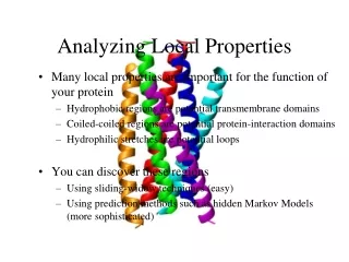
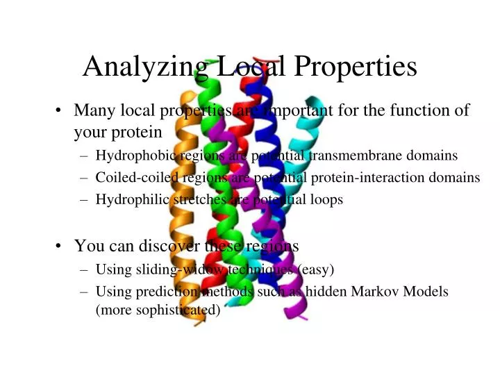
Analyzing Local Properties. Many local properties are important for the function of your protein Hydrophobic regions are potential transmembrane domains Coiled-coiled regions are potential protein-interaction domains Hydrophilic stretches are potential loops You can discover these regions

E N D
Analyzing Local Properties • Many local properties are important for the function of your protein • Hydrophobic regions are potential transmembrane domains • Coiled-coiled regions are potential protein-interaction domains • Hydrophilic stretches are potential loops • You can discover these regions • Using sliding-widow techniques (easy) • Using prediction methods such as hidden Markov Models (more sophisticated)
Sliding-window Techniques • Ideal for identifying strong signals • Very simple methods • Few artifacts • Not very sensitive • Use ProtScale on www.expasy.org • Make the window the same size as the feature you’re looking for
www.expasy.org/cgi-bin/protscale.pl Hphob. / Eisenberg
Using TMHMM • TMHMM is the best method for predicting transmembrane domains • TMHMM uses an HMM • Its principle is very different from that of ProtScale • TMHMM output is a prediction
Searching for PROSITE Patterns • Search your protein against PROSITE on ExPAsy • www.expasy.org/tools/scanprosite • PROSITE motifs are written as patterns • Short patterns are not very informative by themselves • They only indicate a possibility • Combine them with other information to draw a conclusion • Remember: Not everything is in PROSITE !
Protein Domains • Proteins are usually made of domains • A domain is an autonomous folding unit • Domains are more than 50 amino acids long • It’s common to find these together: • A regulatory domain • A binding domain • A catalytic domain
Secondary Structures • Helix • Amino acid that twists like a spring • Beta strand or extended • Amino acid forms a line without twisting • Random coils • Amino acid with a structure neither helical nor extended • Amino-acid loops are usually coils
Servers • www.predictprotein.org • cubic.bioc.columbia.edu/predictprotein • www.sdsc.edu/predicprotein • www.cbi.pku.edu.cn/predictprotein
Introduction • R is: • a suite of operators for calculations on arrays, in particular matrices, • a large, coherent, integrated collection of intermediate tools for interactive data analysis, • graphical facilities for data analysis and display either directly at the computer or on hardcopy • a well developed programming language which includes conditionals, loops, user defined recursive functions and input and output facilities. • The core of R is an interpreted computer language. • It allows branching and looping as well as modular programming using functions. • Most of the user-visible functions in R are written in R, calling upon a smaller set of internal primitives. • It is possible for the user to interface to procedures written in C, C++ or FORTRAN languages for efficiency, and also to write additional primitives.
R and statistics • Packaging: a crucial infrastructure to efficiently produce, load and keep consistent software libraries from (many) different sources / authors • Statistics: most packages deal with statistics and data analysis • State of the art: many statistical researchers provide their methods as R packages
Data Analysis and Presentation • The R distribution contains functionality for large number of statistical procedures. • linear and generalized linear models • nonlinear regression models • time series analysis • classical parametric and nonparametric tests • clustering • smoothing • R also has a large set of functions which provide a flexible graphical environment for creating various kinds of data presentations.
R as a calculator > log2(32) [1] 5 > sqrt(2) [1] 1.414214 > seq(0, 5, length=6) [1] 0 1 2 3 4 5 > plot(sin(seq(0, 2*pi, length=100)))
Object orientation • primitive (or: atomic) data types in R are: • numeric (integer, double, complex) • character • logical • function • out of these, vectors, arrays, lists can be built.
Object orientation • Object: a collection of atomic variables and/or other objects that belong together • Example: a microarray experiment • probe intensities • patient data (tissue location, diagnosis, follow-up) • gene data (sequence, IDs, annotation) • Parlance: • class: the “abstract” definition of it • object: a concrete instance • method: other word for ‘function’ • slot: a component of an object
Object orientation Advantages: Encapsulation (can use the objects and methods someone else has written without having to care about the internals) Generic functions (e.g. plot, print) Inheritance (hierarchical organization of complexity) Caveat: Overcomplicated, baroque program architecture…
variables > a = 24 > b<-25 > sqrt(a+b) [1] 7 > a = "The dog ate my homework" > sub("dog","cat",a) [1] "The cat ate my homework" > a = (1+1==3) > a [1] FALSE numeric character string logical
variables > paste("X", "Y") > paste("X", "Y", sep = " + ") > paste("Fig", 1:4) > paste(c("X", "Y"), 1:4, sep = "", collapse = " + ")
x<-2.17 y<-as.character(x) z<-as.numeric(y) Help(as)
vectors, matrices and arrays • vector: an ordered collection of data of the same type • > a = c(1,2,3) • > a*2 • [1] 2 4 6 • Example: the mean spot intensities of all 15488 spots on a chip: a vector of 15488 numbers • In R, a single number is the special case of a vector with 1 element. • Other vector types: character strings, logical
vectors, matrices and arrays • matrix: a rectangular table of data of the same type • example: the expression values for 10000 genes for 30 tissue biopsies: a matrix with 10000 rows and 30 columns. • array: 3-,4-,..dimensional matrix • example: the red and green foreground and background values for 20000 spots on 120 chips: a 4 x 20000 x 120 (3D) array.
Lists • vector: an ordered collection of data of the same type. • > a = c(7,5,1) • > a[2] • [1] 5 • list: an ordered collection of data of arbitrary types. > doe = list(name="john",age=28,married=F) • > doe$name • [1] "john " • > doe$age • [1] 28 • Typically, vector elements are accessed by their index (an integer), list elements by their name (a character string). But both types support both access methods.
Data frames data frame: is like a spreadsheet. It is a rectangular table with rows and columns; data within each column has the same type (e.g. number, text, logical), but different columns may have different types. Example: > a localisation tumorsize progress XX348 proximal 6.3 FALSE XX234 distal 8.0 TRUE XX987 proximal 10.0 FALSE
id<-c("xx348", "xx234", "xx987") locallization<-c("proximal", "distal", "proximal") progress<-c(F, T, F) tumorsize<-c(6.3, 8.0, 10.0) results<-data.frame(id, locallization , tumorsize, progress) > results id locallization tumorsize progress 1 xx348 proximal 6.3 FALSE 2 xx234 distal 8.0 TRUE 3 xx987 proximal 10.0 FALSE
> summary(results) id locallization tumorsize progress xx234:1 distal :1 Min. : 6.30 Mode :logical xx348:1 proximal:2 1st Qu.: 7.15 FALSE:1 xx987:1 Median : 8.00 TRUE :2 Mean : 8.10 NA's :0 3rd Qu.: 9.00 Max. :10.00 >x<-summary(results) >x id locallization tumorsize progress xx234:1 distal :1 Min. : 6.30 Mode :logical xx348:1 proximal:2 1st Qu.: 7.15 FALSE:1 xx987:1 Median : 8.00 TRUE :2 Mean : 8.10 NA's :0 3rd Qu.: 9.00 Max. :10.00
Subsetting Individual elements of a vector, matrix, array or data frame are accessed with “[ ]” by specifying their index, or their name > results localisation tumorsize progress XX348 proximal 6.3 0 XX234 distal 8.0 1 XX987 proximal 10.0 0 > results[3, 2] [1] 10 > a["XX987", "tumorsize"] [1] 10 > results["XX987",] localisation tumorsize progress XX987 proximal 10 0
> results localisation tumorsize progress XX348 proximal 6.3 0 XX234 distal 8.0 1 XX987 proximal 10.0 0 > results[c(1,3),] localisation tumorsize progress XX348 proximal 6.3 0 XX987 proximal 10.0 0 > results[c(T,F,T),] localisation tumorsize progress XX348 proximal 6.3 0 XX987 proximal 10.0 0 > results$localisation [1] "proximal" "distal" "proximal" > results $localisation=="proximal" [1] TRUE FALSE TRUE > results[ results$localisation=="proximal", ] localisation tumorsize progress XX348 proximal 6.3 0 XX987 proximal 10.0 0 Subsetting subset rows by a vector of indices subset rows by a logical vector subset a column comparison resulting in logical vector subset the selected rows
results[2,] results[2,2] results[1:3,] results[c(1,3),] results[c(T,F,T),] x<-summary(results) x X[2,2]
x = c(1, 1, 2, 3, 5, 8) x[c(TRUE, TRUE, FALSE, FALSE, TRUE, TRUE)] x[c(TRUE, FALSE)] x == 1 x[x == 1] x[x%%2 == 0] y = c(1, 2, 3) y[]=3 y
Matrix • a matrix is a vector with an additional attribute (dim) that defines the number of columns and rows • only one mode (numeric, character, complex, or logical) allowed • can be created using matrix() x<-matrix(data=0,nr=2,nc=2) or x<-matrix(0,2,2)
Data Frame • several modes allowed within a single data frame • can be created using data.frame() L<-LETTERS[1:4] #A B C D x<-1:4 #1 2 3 4 data.frame(x,L) #create data frame • attach() and detach() • the database is attached to the R search path so that the database is searched by R when it is evaluating a variable. • objects in the database can be accessed by simply giving their names
a=matrix(1:9, ncol = 3, nrow = 3) a b=matrix(c(TRUE, FALSE, TRUE), ncol = 3, nrow = 3) b x=1:10 y=11:20 z=matrix(c(x,y)) z z=matrix(c(x,y),nrow=2) z z=matrix(c(x,y),nrow=4) z
R code max(z) min(z) length(z) mean(z) sd(z) sum(z)