Download
1 / 76
780 likes | 1.22k Views
Predicate Calculus. Calculus. What does calculus mean? Comes from the word “ stone ” Implies a process of calculating Lots of calculus studies … Differential calculus Integral calculus Relational calculus Propositional calculus Predicate calculus

E N D
Calculus • What does calculus mean? • Comes from the word “stone” • Implies a process of calculating • Lots of calculus studies … • Differential calculus • Integral calculus • Relational calculus • Propositional calculus • Predicate calculus • Predicate calculus is a generalization of propositional calculus Kidney stone
Predicate Calculus • Also called Predicate or First-Order Logic • Contains all of the components of propositional calculus… • Together with: • Predicates • Auniverse of discourse (UofD) • Terms • Quantifiers
Predicates • A predicate is a statement that is either true or false and has zero or more arguments • A predicate has a name followed by a list of arguments enclosed in parentheses and is called an atomic formula Examples: Jane is the mother of Mary isMother(Jane, Mary) M(j, m) • Atomic formulas can be combined by logical connectives Example: isMother(Jane,Mary) isMother(Mary,Jane) • If all arguments of a predicate are individual constants, the resulting atomic formula must either be true or false Examples: Jane is the mother of Mary = T isMother(Jane, Mary) = T isMother(Mary, Jane) = F • The number and order of predicate arguments is significant • The number of elements in the predicate list is called the arity of the predicate
UofD, Terms, Quantifiers • The Universe of Discorse (UofD) is a set of values • The UofD represents all values being considered • The UofD is sometimes called the domain of interest, or simply the domain • Arguments in predicates can be constants (values in the UofD), variables (whose value assignments come from the UofD), or terms (expressions that evaluate to values in the UofD) • Quantifiers give us a way to evaluate predicate calculus formulas with variables that range over the entire UofD Chapter 2, Section 1
UoD = {Jim, Sally, Sara, Zed} siblingOf(x,y) siblingOf Jim Sally Sara Zed Jim F F T T Sally F F F F Sara T F F T Zed T F T F Predicate Evaluation (I) • Sometimes we know the “meaning” but we don’t know which assignments hold until we are told • For example:
UoD = {a, b, c} Facts: P(b, c) P(c, a) P(a, c) P a b c P(x, y) a F F T b F F T c T F F Predicate Evaluation (II) • Sometimes we don’t know the “meaning” but we are “given” the assignments • For example: • Under a “closed world assumption,” we only need to list the facts (substitutions that evaluate to True). All others are False.
Instantiation • Instantiation is the substitution of a constant for a variable (or in general, the substitution of a term, which is an expression that yields a constant) • SxtA means substitute term t for all variables x in A • SxtA is called an instantiation of A and t is said to be an instance of x • Examples: Sx3 P(x, y) = P(3, y) Sx3+1 P(x, y, z, x) = P(3+1, y, z, 3+1) = P(4, y, z, 4)
Universal Quantification (I) • Let A be an expression, and let x be a variable. If we want to say that P(x) is true for all substitutions of values for x in the UofD, we write xP(x). • The symbol is pronounced “for all” and is called the universal quantifier. • Examples: • All cats have tails, x(cat(x) hasTail(x)). • For every integer x, x+1 > x, x(>(x+1, x)).
Universal Quantification (II) • x P(x) is shorthand for: • xP(x) = P(a) P(b) P(c) with UoD = {a, b, c}. • xP(x) = P(0) P(1) … with UoD = non-negative integers. • xP(x) = T when P(x) = T for all substitutions from the UoD. (Only need one false predicate instantiation to make the formula false.) • Examples: • xred(x) = T for UoD = red apples • xred(x) = F for UoD = apples
Existential Quantification (I) • Let A be an expression, and let x be a variable. If we want to say that P(x) is true for at least one value of x, we write xP(x). • The symbol is pronounced “there exists” and is called the existential quantifier. • Examples: • Some people like apples, x(likesApples(x)). • There is an integer larger than 10, x(>(x, 10)).
Existential Quantification (II) • x is shorthand for: • xP(x) = P(a) P(b) P(c) with UoD = {a, b, c}. • xP(x) = P(1) P(2) … with UoD = non-negative integers. • xP(x) = T when P(x) = T for one or more substitutions from UoD. (Only need one true predicate instantiation to make the formula true.) • Examples: • xred(x) = T for UoD = all apples • xred(x) = F for UoD = golden delicious apples
Expressions with Quantifiers • Quantifiers associate right to left. • Example with UoD = {Ann, Sue, Tim} xy loves(x, y) = (x(y(loves(x, y)))) = x(loves(x, Ann) loves(x, Sue) loves(x, Tim)) = (loves(Ann, Ann) loves(Ann, Sue) loves(Ann, Tim)) (loves(Sue, Ann) loves(Sue, Sue) loves(Sue, Tim)) (loves(Tim, Ann) loves(Tim, Sue) loves(Tim, Tim)) • We say, for every x, there exists a y such that x loves y. (Everybody loves somebody.)
Examples • What about yx loves(x, y)? • There exists a y such that for every x, x loves y. • Somebody is loved by everybody. • Not the same as everybody loves somebody. • What about xy loves(x, y)? • There exists an x such that for every y, x loves y. • Somebody loves everybody. • What about yx loves(x, y)? • For every y there exists an x such that x loves y. • Everybody is loved by somebody. • Order matters.
Precedence Quantifiers have the highest precedence: (unary operators) yx P(x, y) Q(x) x R(x, y, z) y (x P(x, y)) Q(x) (x R(x, y, z)) (y (x P(x, y))) Q(x) ((x R(x, y, z))) (y (x P(x, y))) (Q(x) ((x R(x, y, z)))) ((y (x P(x, y))) (Q(x) ((x R(x, y, z)))))
Scope, Bound, and Free • Scope defines extent. Parentheses define scope, and precedence dictates how to insert parentheses. • Bound variables define “sameness”. • A variable is bound if it “is introduced by” a quantifier. • A variable remains bound throughout the scope of the quantifier unless rebound by another quantifier in a nested sub formula. • Any variable that is not bound is said to be free. • We can consider bound variables to be local to the scope of the quantifier, just as parameters and locally declared variables in procedures are local to the procedure in which they are declared. • If several quantifiers use the same bound variable for quantification, then all those variables are local to their scope and are distinct.
Example Which variables are bound and which are free? y x (P(x, y) (Q(x) x R(x, y, z)))
Example Which variables are bound and which are free? y x (P(x, y) (Q(x) x R(x, y, z))) y is bound x is bound x is bound z is free different x’s
Providing Meaning • Consider the problem of giving meaning to the expression: sibling(x, Lynn) married(x). • Can’t just assign T or F to a predicate expression with variables • Truth depends on the values assigned to the variables • E.g., assign Zed to x; then if Zed is indeed Lynn’s sibling and is married, we can say that this expression is true. • E.g., for x(sibling(x, Lynn) married(x)), we can look through the list of all possibilities (i.e. look through the domain) and see if at least one of them is a sibling of Lynn and is married; if so we can say that this expression is true. • To provide an interpretation, we need • A domain that provides values for the arguments of the predicate • A way to determine the truth value of all predicates for each possible assignment of domain values to the variables
Interpretation (I) • An interpretation for an expression E • Specify a domain, D. • For each predicate of E, specify T or F for every possible substitution. • Select a value in D for each free variable, if any. • Example: yP(x, y) D = {1, 2} P(x, y) = ? 1 1 T 1 2 F 2 1 F 2 2 F x = 1: yP(x, y) = P(1, 1) P(1, 2) = T F = T x = 2: yP(x, y) = P(2, 1) P(2, 2) = F F = F
Interpretation (II) • An interpretation for an expression E • Specify a domain, D. • For each predicate of E, specify T or F for every possible substitution. • Select a value in D for each free variable, if any. • Example: yP(x, y) D = {1, 2} P(x, y) = ? 1 1 T 1 2 F 2 1 T 2 2 F x = 1: yP(x, y) = P(1, 1) P(1, 2) = T F = T x = 2: yP(x, y) = P(2, 1) P(2, 2) = T F = T Observe that the truth of a statement depends on the interpretation.
Interpretation (III) • An interpretation for an expression E • Specify a domain, D. • For each predicate of E, specify T or F for every possible substitution. • Select a value in D for each free variable, if any. • Example: xyP(x, y) D = {1, 2} P(x, y) = ? 1 1 T 1 2 F 2 1 F 2 2 F xyP(x, y) = x(P(x, 1) P(x, 2)) = (P(1, 1) P(1, 2)) (P(2, 1) P(2, 2)) = (T F) (F F) = T F = F
Interpretation (IV) • An interpretation for an expression E • Specify a domain, D. • For each predicate of E, specify T or F for every possible substitution. • Select a value in D for each free variable, if any. • Example: xyP(x, y) D = {1, 2} P(x, y) = ? 1 1 T 1 2 F 2 1 T 2 2 F xyP(x, y) = x(P(x, 1) P(x, 2)) = (P(1, 1) P(1, 2)) (P(2, 1) P(2, 2)) = (T F) (T F) = T T = T
Closed World Assumption • With the closed world assumption, we only give the substitutions that evaluate to true — all others are assumed to be false. • Let the domain, D = {1, 2}, then if we write: P(x, y) or P(1, 1) 1 1 P(1, 2) 1 2 • Then with the closed world assumption, this is simply shorthand for writing: P(x, y) = ? or 1 1 T P(1, 1) = T 2 1 F P(2, 1) = F 1 2 T P(1, 2) = T 2 2 F P(2, 2) = F
Closed World Assumption Notes • Our project uses the closed world assumption. • Only the substitutions that hold are given. • These are called facts. • Real-world databases use the closed world assumption only “true” facts are stored. • Contrary to the closed world assumption, the open world assumption says that if a fact is not stated, we do not know whether it is true or false. • The open world assumption is typical in everyday life. • It is harder to work with an open world assumption.
Schemes: snap(S,N,A,P) csg(C,S,G) cp(C,Q) cdh(C,D,H) cr(C,R) Facts: snap('12345','C. Brown','12 Apple St.','555-1234'). snap('67890','L. Van Pelt','34 Pear Ave.','555-5678'). snap('22222','P. Patty','56 Grape Blvd.','555-9999'). snap('33333','Snoopy','12 Apple St.','555-1234'). csg('CS101','12345','A'). csg('CS101','67890','B'). csg('EE200','12345','C'). csg('EE200','22222','B+'). csg('EE200','33333','B'). csg('CS101','33333','A-'). csg('PH100','67890','C+'). cp('CS101','CS100'). cp('EE200','EE005'). cp('EE200','CS100'). cp('CS120','CS101'). cp('CS121','CS120'). cp('CS205','CS101'). cp('CS206','CS121'). cp('CS206','CS205'). cdh('CS101','M','9AM'). cdh('CS101','W','9AM'). cdh('CS101','F','9AM'). cdh('EE200','Tu','10AM'). cdh('EE200','W','1PM'). cdh('EE200','Th','10AM'). cdh('PH100','Tu','11AM'). cr('CS101','Turing Aud.'). cr('EE200','25 Ohm Hall'). cr('PH100','Newton Lab.'). Rules: WhoGradeCourse(N,G,C):-csg(C,S,G),snap(S,N,A,P). before(C1,C2):-cp(C2,C1). before(C1,C2):-cp(C3,C1),before(C3,C2). Queries: WhoGradeCourse('Snoopy',G,C)? WhoGradeCourse(N,'A','CS100')? WhoGradeCourse(N,'A',C)? before('CS100','CS206')? before('CS100',X)?
Example #1 (Class Project) • Query: What are the prerequisites of EE200? • Translated to predicate logic, we are asking for: cp('EE200', x) where: cp(course, prerequisite) • We need to find the substitutions for the free variable x, if any, that make this true. • Interpretation for the project: • Domain = all constant strings in the Facts • Closed world assumption holds (if stated as a fact, then T; otherwise, F).
Example #1 (cont’d) cp Facts: cp('CS101','CS100'). cp('EE200','EE005'). cp('EE200','CS100'). cp('CS120','CS101'). cp('CS121','CS120'). cp('CS205','CS101'). cp('CS206','CS121'). cp('CS206','CS205'). • Check all substitutions for cp('EE200', x) from the domain for x: cp('EE200','10AM') = F cp('EE200','11AM') = F cp('EE200','12 Apple St.') = F … cp('EE200','CS100') = T x = 'CS100' … cp('EE200','EE005') = T x = 'EE005' … • Also, • x cp('EE200', x) = T • x cp('EE200', x) = F • x cp('CS100', x) = F Note: Untyped Logic
Example #2 (Class Project) • Query: Where am I likely to find Charlie Brown ('12345') on Wednesday ('W') at 1 PM ('1PM')? • Translated to predicate logic, we are asking for: xz(csg(x,'12345',z) cr(x,r) cdh(x,'W','1PM')) where: csg(course, studentID, grade) cr(course, room) cdh(course, day, hour) ris a free variable
Example #2 (cont’d) Check substitutions for all combinations of values from the domain for x, z, and r: … csg('10AM','12345','10AM') cr('10AM','10AM') cdh('10AM','W','1PM') = F csg('10AM','12345','10AM') cr('10AM','11AM') cdh('10AM','W','1PM') = F csg('10AM','12345','10AM') cr('10AM','12 Apple St.') cdh('10AM','W','1PM') = F … csg('10AM','12345','11AM') cr('10AM','10AM') cdh('10AM','W','1PM') = F csg('10AM','12345','11AM') cr('10AM','11AM') cdh('10AM','W','1PM') = F csg('10AM','12345','11AM') cr('10AM','12 Apple St.') cdh('10AM','W','1PM') = F … csg('11AM','12345','10AM') cr('11AM','10AM') cdh('11AM','W','1PM') = F csg('11AM','12345','10AM') cr('11AM','11AM') cdh('11AM','W','1PM') = F csg('11AM','12345','10AM') cr('11AM','12 Apple St.') cdh('11AM','W','1PM') = F … csg('11AM','12345','11AM') cr('11AM','10AM') cdh('11AM','W','1PM') = F csg('11AM','12345','11AM') cr('11AM','11AM') cdh('11AM','W','1PM') = F csg('11AM','12345','11AM') cr('11AM','12 Apple St.') cdh('11AM','W','1PM') = F …
Example #2 (cont’d) csg, cdh, and cr Facts: csg('CS101','12345','A'). csg('CS101','67890','B'). csg('EE200','12345','C'). csg('EE200','22222','B+'). csg('EE200','33333','B'). csg('CS101','33333','A-'). csg('PH100','67890','C+'). cdh('CS101','M','9AM'). cdh('CS101','W','9AM'). cdh('CS101','F','9AM'). cdh('EE200','Tu','10AM'). cdh('EE200','W','1PM'). cdh('EE200','Th','10AM'). cdh('PH100','Tu','11AM'). cr('CS101','Turing Aud.'). cr('EE200','25 Ohm Hall'). cr('PH100','Newton Lab.'). • Eventually, we check the substitution x = 'EE220',z = 'C',and r = '25 Ohm Hall'. csg('EE220','12345','C') cr('EE220','25 Ohm Hall') cdh('EE220','W','1PM') = T • Thus, Charlie Brown is likely to be in 25 Ohm Hall on Wednesday at 1 PM.
Validity • An expression that is true for all interpretations is said to be valid. (A valid expression is also call a tautology.) • An expression that is true for no interpretation is said to be contradictory. (A contradictory expression is also called a contradiction.) • If A is valid, A is contradictory. (a tautology) (a contradiction) • Examples: • P(x, y) P(x, y) P(x, y) P(x, y) is valid • P(x, y) P(x, y) is contradictory Laws are valid!
DeMorgan’s Laws with Quantifiers deMorgan’slaws: xA xA xA xA Proof: xP(x) (P(x1) P(x2) …) P(x1) P(x2) … xP(x)
An expression with the variable names changed is called a variant. Proper variants are equivalent, i.e., it doesn’t matter what variable name is used. Example: xA ySxyA But, we must be careful We must substitute only for the x’s bound by x. Further, variables must not “clash.” Strong rule: y must not be in A; weaker rule: no y in the scope of x can be free in the scope of x, and no x bound by x may be in the scope of a bound y. x(y(P(y) Q(x,z)) xP(x)) Renaming w w Works z z Doesn’t work y y Doesn’t work x(yP(y) Q(x,z)) xP(x) y yWorks
free free same free Rectification Standardizing variables apart, also called rectification we can rename variables to make distinct variables have distinct names. (xP(x, y) xQ(y, x)) yR(y, x) (xP(x, y) zQ(y, z)) wR(w, v)
Universal Instantiation (UI) When A is true for every instantiation, it is certainly true for some particular instantiation xA SxtA Example: from x Mortal(x), we can derive Mortal(Smith)
Existential Instantiation (EI) When A is true for one or more instantiations, we can let a variable, say b, designate any one of the true instantiations. xA SxbA Example: from x Mortal(x), we can derive Mortal(b), where b is a variable that stands for somebody who is mortal. Caution: Because we don’t know which one(s) in the domain make A hold, we must make sure b is a new variable not one already in use. For example, if we have x Succeeds(x) and x Fails(x), then we cannot conclude Succeeds(b) and Fails(b) the first b is OK, but not the second.
Existential Generalization (EG) SxtA xA If we know A is true for some particular substitution t, we know there exists at least one substitution for which A is true.
Universal Generalization (UG) A xA If A holds with no restrictions on one of its variables x, it must hold for all substitutions for x. Example: from x(P(x) Q(x)) and xP(x), we can conclude P(a) Q(a) and P(a) by UI and then Q(a) by modus ponens; and thus by UG we can conclude xQ(x). Careful: from x<100, we cannot infer x x>100 by UG
Derivation Example If xyz(Q(x, y) P(z)), wP(w) then xQ(x, 8). • xyz(Q(x, y) P(z)) premise • Q(a, b) P(c) 1, UI Sxa, Syb, Szc • P(c) Q(a, b) 2, contrapositive • wP(w) premise • P(c) 4, UI Swc • Q(a, b) 3&5, modus ponens • xyQ(x, y) 6, UG (Neither a nor b is free in a premise, nor were they introduced by EI) • xQ(x, 8) 7, UI Sy8 Note: in Step 2, we could have used Sxx, Syy, Szz: the names of the variables don’t matter, so long as we follow the rules properly
Unification The previous proof was basically about getting rid of universal quantifiers and then reintroducing them and about getting the variable names to match for modus ponens and for the conclusion. Since, we “play this game” over and over, we could (and should) simplify by doing two things: 1. Drop initial ’s, so long as we remember which variables are actually bound to these universal quantifiers so that we use them properly and which variables (if any) are fixed in the premises. 2. Use unification. Two expressions unify if there are legal instantiations that make them the same.
Simplified Derivation Example If Q(x, y) P(z), P(w) then Q(x, 8). • Q(x, y) P(z) premise • P(z) Q(x, y) 1, contrapositive • P(w) premise • P(z) 3, unification with 2 • Q(x, y) 2&4, modus ponens • Q(x, 8) 5, instantiation Informally, we can see that this works: If 2 & 3 are true for all substitutions, then we can always choose the w to be the same as z and be guaranteed that they will both be true (assuming the premises are true). Note that the UI and UG are “hidden” within the unification
Programming a Computer to do Proofs Too much work to program all the possibilities we have considered. We need a better way. • Better = more uniform not so many cases (even though it may sometimes be longer). • Better = fewer rules of inference. • Better = a heuristic guide to lead us to the conclusion. • Better = easier to convert to an algorithm.
Consider… Prove that this rule of inference is valid. P A P B A B
P A B (P A) (P B) A B T T T T T F T T T T T F T F F F T T T F T T T F T T T T F F T F F F T F F T T T T T T T T F T F T T T T T T F F T F F T T T T F F F F F T T T F It is Valid
Using your new rule, rewrite Modus ponens Modus tollens Hypothetical syllogism P Q Q R P R P Q P Q P P Q Q P F P Q Q F P F Q P Q F P Q Q R P R We now have one rule to rule them all!