Download
1 / 22
220 likes | 365 Views
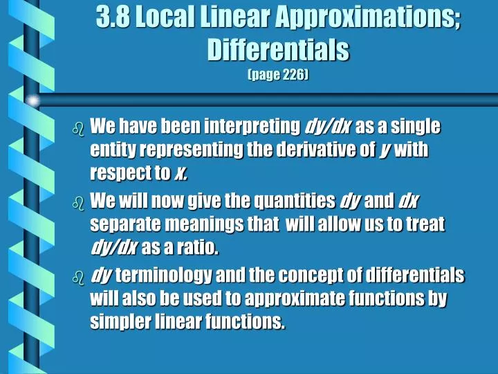
3.8 Local Linear Approximations; Differentials (page 226). We have been interpreting dy/dx as a single entity representing the derivative of y with respect to x. We will now give the quantities dy and dx separate meanings that will allow us to treat dy/dx as a ratio.

E N D
3.8 Local Linear Approximations;Differentials(page 226) • We have been interpreting dy/dx as a single entity representing the derivative of y with respect to x. • We will now give the quantities dy and dx separate meanings that will allow us to treat dy/dx as a ratio. • dy terminology and the concept of differentials will also be used to approximate functions by simpler linear functions.
Historical Note(See page 4) Isaac Newton (1642-1727) • Woolsthorpe, England • Not gifted as a youth • Entered Trinity College with a deficiency in geometry. • 1665 to 1666 - discovered Calculus • Calculus work not published until 1687 • Viewed value of work to be its support of the existence of God.
Historical Note(See page 5) Gottfried Wilhelm Leibniz (1646-1716 • Leipzig, Germany • Gifted Genius • Entered University of Altdorf at age 15 • Doctorate by age 20 • Developed Calculus in 1676 • Developed the dy/dx notation we use today
Example / Not in this edition
Local Linear Approximation(page 226) • If the graph of a function is magnified at a point “P” that is differentiable, the function is said to be locally linear at “P”. • The tangent line through “P” closely approximates the graph. • A technique called “ local linear approximation” is used to evaluate function at a particular value.
Locally Linear Function at a Differentiable Point “P”(page 226)
Function Not Locally Linear at Point “P” Because Function Not Differentiable at Point “P”
Error Propagation in Applications(page 230) • In applications small errors occur in measured quantities. • When these quantities are used in computations, those errors are “propagated” throughout the calculation process. • To estimate the propagated error use the formula below: