Download
1 / 17
170 likes | 294 Views
Simplifying Dynamic Programming via Tabling. Hai-Feng Guo University of Nebraska at Omaha, USA Gopal Gupta University of Texas at Dallas, USA. Tabled Logic Programming. A tabled logic programming system terminate more often by computing fixed points

E N D
Simplifying Dynamic Programming via Tabling Hai-Feng Guo University of Nebraska at Omaha, USA Gopal Gupta University of Texas at Dallas, USA
Tabled Logic Programming • A tabled logic programming system • terminate more often by computing fixed points • avoid redundant computation by memoing the computed answers • Keeps the declarative and procedural semantics consistent for any definite logic programs. • Tabled resolution schemes • OLDT, SLG, SLS, SLDT, DRA
:- table reach/2 reach(X, Y) :- reach(X, Z), arc(Z, Y). reach(X, Y) :- arc(X, Y). arc(a, b). arc(b, a). arc(b, c). :- table reach/3 reach(X, Y, E) :- reach(X, Z, E1), arc(Z, Y, E2), append(E1, E2, E). reach(X, Y, E) :- arc(X, Y, E). arc(a, b, [(a, b)]). arc(b, a, [(b, a)]). arc(b, c, [(b, c)]). Reachability a b c Table Space will be increased dramatically due to the extra argument to record the path.
How tabled answers are collected? • When an answer to a tabled call is generated, variant checking is used to check whether it has been already tabled. • Observation: for collecting paths for the reachability problem, we need only one simple path for each pair of nodes. A second possible path for the same pair of nodes could be thought of as a variant answer.
Indexed / Non-indexed • The arguments of each tabled predicate are divided into indexed and non-indexed ones. • Only indexed arguments are used for variant checking for collecting tabled answers. • Non-indexed arguments are treated as no difference.
Mode Declaration for Tabled Predicates :- table_mode p(a1, …, an). • p/n is a predicate name, n > 0; • each ai has one of the following forms: • + denotes that this indexed argument is used for variant checking; • denotes that this non-indexed arguments is not be used for variant checking; • * denotes that they are always bound before a call to the tabled predicate p/n is invoked.
Aggregate Declaration • Associate a non-indexed argument of a tabled predicate with some optimum constraint, e.g. minimum or maximum. • The argument mode also includes: • 0 denotes that this argument is a minimum; • 9 denotes that this argument is a maximum.
Dynamic Programming • Dynamic programming is typically used for solving optimization problems. • A recursive strategy: the value of an optimal solution is recursively defined in terms of optimal solutions to sub-problems.
Dynamic Programming with Mode declaration • Optimization = Problem + Aggregation • With mode declaration, defining a general solution suffices.
Matrix-Chain Multiplication Without Mode Declaration With Mode Declaration
Matrix-Chain Multiplication :- table scalar_cost/4. :- table_mode scalar_cost(+, 0, , ). scalar_cost([P1, P2], 0, P1, P2). scalar_cost([P1, P2, P3 | Pr], V, PL1, PL2) :- break([P1, P2, P3 | Pr], PL1, PL2, Pk), scalar_cost(PL1, V1, P1, Pk), scalar_cost(PL2, V2, Pk, Pn), V is V1 + V2 + P1 * Pk * Pn.
Running Time Comparison (Seconds) Without Evidence Construction With Evidence Construction • The programs with mode declaration run 1.34 to 16.0 times faster than those without mode declaration.
Scalability Without Evidence With Evidence
Running Space Comparison (Megabytes) Without Evidence Construction • Without evidence construction, the programs with mode declaration consumes 1.4 to 15.0 times less space than those without mode declaration.
Running Space Comparison (Megabytes) With Evidence Construction • With evidence construction, space performance can be better or worse depending on the programs. • The programs without mode explicitly generate all possible answers and then table the optimal one; • The programs with mode implicitly generate all possible answers and selectively table the better answers until the optimal one is found.
Conclusion • A new mode declaration for tabled predicates is introduced to aggregate information dynamically recorded in the table; • A tabled predicate can be regarded as a function in which non-indexed arguments (outputs) are uniquely defined by the indexed arguments (inputs); • The new mode declaration scheme, coupled with recursion, provides an elegant method for solving optimization problems; • The efficiency of tabled resolution is improved since only indexed arguments are involved in variant checking.