Citations

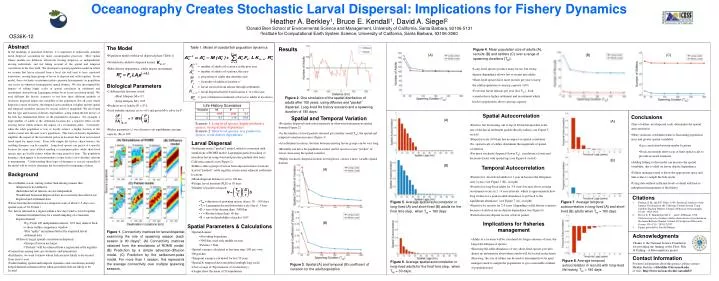
1. Oceanography Creates Stochastic Larval Dispersal: Implications for Fishery Dynamics Heather A. Berkley1, Bruce E. Kendall1,David A. Siegel2 1Donald Bren School of Environmental Science and Management, University of California, Santa Barbara, 93106-5131 2Institute for Computational Earth System Science, University of California, Santa Barbara, 93106-3060 OS36K-12 Abstract In the modeling of nearshore fisheries, it is important to realistically simulate larval dispersal, accounting for many oceanographic processes. Most spatial fishery models use diffusion, effectively treating dispersers as independently moving individuals, and not taking account of the spatial and temporal correlations in the flow field. We developed a spatial population model in which we assume that larvae released from a local site will tend to have correlated trajectories, causing large groups of larvae to disperse and settle together. In our model, these stochastic recruitment pulses generate heterogeneity in population size across an otherwise homogeneous spatial domain. We also investigated the impacts of adding larger scales of spatial correlation in settlement and recruitment, derived from Lagrangian studies by an ocean circulation model. We used different life history scenarios to test how these different methods of stochastic dispersal impact the variability of the population. For all cases where dispersal is more stochastic, the temporal autocorrelation is higher and the spatial and temporal variability increase by several orders of magnitude. We also found that the type and location of density dependence, acting within the life history of the fish, has fundamental effects on the population’s dynamics. For example, a large number of adults at the settlement location has a negative effect on the arriving larvae which reduces the impact of a recruitment pulse. Conversely, when the adult population is low or locally extinct, a higher fraction of the settlers recruit into the next year’s population. This form of density dependence amplifies the impact of the recruitment pulses in locations that have not received larval input for many years. Even with simple life history characteristics, the resulting dynamics can be complex. Long-lived species can persist at a specific location for many years without needing a recruitment pulse, while short-lived species may go locally extinct within the same period of time. The population dynamics often appear to be nonstationary at time scales (a few decades) relevant to management. Understanding these types of dynamics is crucial, especially if the model will be used to determine the best method for managing a fishery. • The Model • Population model with larval dispersal phase (Table 1) • Stochasticity added to dispersal kernel, • Riker density dependence, adults impact recruitment Table 1. Model of coastal fish population dynamics Results Figure 4. Mean population size of adults (A), recruits (B) and settlers (C) over a range of spawning durations (Tsp). (A) (B) (C) • Long-lived species produce many larvae, but strong density dependence allows few to recruit into adults • Short-lived species have more recruits per year to keep the adult population at carrying capacity (100) • For fewer larval releases per year (low Tsp ), both scenarios have higher settlement and recruitment which leads to populations above carrying capacity = number of adults at location x in the next year = number of adults at location x this year = proportion of adults that died this year = fecundity of adults at location x’ = larval survival (from release through settlement) = larval dispersal kernel from location x’ to x this year = post-settlement recruitment of larvae to adults at location x • Biological Parameters • 2 different life histories tested • Short lifespan, M = 0.5 • Long lifespan, M = 0.05 • Productivity of Adults (P) = F*L • Used stability analysis set to +0.5 and given M to solve for P: • Ricker parameter (c) was chosen to set equilibrium carrying capacity (K) at 100 Figure 2. One simulation of the spatial distribution of adults after 100 years, using diffusive and “packet” dispersal. Long-lived life history scenario and a spawning duration of 180 days. • Spatial Autocorrelation • Positive, but decreasing, out to lag of 40 km because this is the size of the larval settlement packet (Rossby radius) (see Figure 5, on left) • Dispersal scale (100 km) has no impact on spatial correlation • So, spatial scale of eddies determines the magnitude of spatial correlation • For more stochastic dispersal (lower Tsp), correlation is lower and decreases faster with spatial lags (see Figure 6, on left) • Conclusions • Size of eddies, not dispersal scale, determines the spatial autocorrelation • More stochastic settlement leads to fluctuating population sizes and greater spatial variability • Less correlation between nearby locations • Stock assessment must occur at finer spatial scale to provide accurate estimates • Adding fishing to this model can increase the spatial variability, due to adult on larvae density dependence • Fishery managers need to know the appropriate space and time scales to sample the fish stocks • Using data without sufficient levels of detail will lead to suboptimal management of the fishery • Spatial and Temporal Variation • Stochastic dispersal creates heterogeneity in otherwise homogeneous spatial domain (Figure 2) • As the number of larval packets released gets smaller (small Tsp), the spatial and temporal variation increases (Figure 3) • At settlement locations, the time between arriving larvae groups can be very long • Mortality can drive the population extinct until it receives a new “packet” of larvae, increasing the spatial variation • Highly stochastic dispersal in short-lived species, creates a more variable spatial domain (A) (A) Scenario 1: Long lived species, highly productive species, strong density dependence Scenario 2:Short lived species, less productive species, weak density dependence • Larval Dispersal • Settlement-pulse (“packet”) model, which is consistent with simulations of ROMS model: Lagrangian particle tracking of nearshore larvae using wind and pressure gradient data from California central coast (Figure 1) • Eddies collect groups of larvae from adjacent release locations • Larval “packets” settle together, across many adjacent settlement locations • Mean dispersal distance is set to 100 km • Pelagic larval duration (PLD) is 50 days • Number of packets released: • Tsp = duration of spawning season (days): 30 – 300 days • Tl = Lagrangian decorrelation time scale (days): 3 days • D = size of the domain (km): 3000 km • r = Rossby radius (km): 40 km • S = survival probability of packet: 0.05 (B) (B) • Temporal Autocorrelation • Positive for short-lived adults for 1 year in because the lifespan is only 2 years (see Figure 7 (B), on right) • Positive for long-lived adults for3-4 years because above average recruitment occurs in 2 - 4 year intervals, which is approximately how long it takes for a peak in adult abundance to get back to the equilibrium abundance (see Figure 7 (A), on right) • Negative for recruits for 2-4 years (depending on life history scenario) because of adult on larvae density dependence (see Figure 8) • Pattern does not depend on size of larval packet (A) • Background • In a turbulent ocean, stirring (rather than mixing) means that: • Dispersal is not diffusive • Individual larval releases are not independent • Traditional Gaussian dispersal does not accurately describe larval dispersal and settlement data • Flows become decorrelated on a temporal scale of about 1-5 days on a spatial scale of 10-50 km1,2 • So, larvae released in a region within a few days tend to travel together • Annual recruitment may be a small sampling of a Gaussian dispersal kernel • E.g. From 100 independent releases, 10% may make it back to shore within competency window • This “spiky” recruitment better fits empirical larval settlement data • If there is larger spatial correlation in dispersal, • Groups of larvae are larger • “Packets” will be released from a region and settle together • Connections among sites are stochastic and intermittent • In fisheries, we want to know where fish are most likely to be located from year to year • Understanding spatial and temporal dynamics and correlation can help keep fishermen informed about when and where fish are likely to be located • Citations • Poulain, P. M. and P. P. Niiler. 1989. Statistical-Analysis of the Surface Circulation in the California Current System Using Satellite-Tracked Drifters. Journal of Physical Oceanography 19(10): 1588-1603. • Dever, E. P., Hendershott M. C., and C.D Winant. 1998. Statistical aspects of surface drifter observations of circulation in the Santa Barbara Channel. Journal of Geophysical Research-Oceans 103(C11): 24781-24797. • Figure provided by Satoshi Mitarai Figure 5. Average spatial autocorrelation in long-lived (A) and short-lived (B) adults for the final time step, when Tsp = 180 days. Figure 7. Average temporal autocorrelation in long-lived (A) and short-lived (B) adults when Tsp = 180 days. (B) • Implications for fisheries management • Adults at a location will be correlated for longer amounts of time, the longer the lifespan of species • Knowing the adult abundance of very short-lived species provides almost no information about where adults will be located in the future • Knowing the size of eddies can be used to determine how far apart managers need to sample the populations to get a reasonable estimate of population size Spatial Parameters & Calculations Figure 1. Connectivity matrices for larval dispersal examining the role of spawning season (each season is 90 days)3. (A) Connectivity matrices obtained from the simulations of ROMS model. (B) Prediction by a simple advection-diffusion model. (C) Prediction by the settlement-pulse model. For more than 1 season, this represents the average connectivity over multiple spawning seasons. • Spatial domain: • Absorbing boundaries • 3000 km, used only middle section • Patches = 5km • Spatial variance calculated at last time step (100 yrs) over 300 patches • Temporal variance calculated for last 50 years • Spatial & temporal autocorrelation (multiple lags each) • Over a range of Tsp (measure of stochasticity) • Graphs show the mean of 50 simulations Acknowledgments Thanks to the National Science Foundation for providing the funding of the Flow, Fish & Fishing – A Biocomplexity project. For more information about this project, please contact Heather Berkley at hberkley@bren.ucsb.edu or visit:http://www.icess.ucsb.edu/~satoshi/f3/ Contact Information Figure 8. Average temporal autocorrelation in recruits with long-lived life history, Tsp = 180 days. Figure 6. Average spatial autocorrelation in long-lived adults for the final time step, when Tsp = 30 days. Figure 3. Spatial (A) and temporal (B) coefficient of variation for the adult population.