Download
1 / 32
330 likes | 519 Views
Differential Expression and False Discovery Rate. Revisiting the Princeton Stem Cell Data GPBA Workshop Oct. 15, 2003. Gene Expression Analysis of Hematopoietic Stem Cells and Committed Progenitors. Hongxian He 1 , Gregory Grant 1 , Lyle Ungar 2 , Natalia B. Ivanova 3 , Ihor R. Lemischka 3 ,

E N D
Differential Expression and False Discovery Rate Revisiting the Princeton Stem Cell Data GPBA Workshop Oct. 15, 2003
Gene Expression Analysis of Hematopoietic Stem Cells and Committed Progenitors Hongxian He1, Gregory Grant1, Lyle Ungar2, Natalia B. Ivanova3, Ihor R. Lemischka3, Chris Stoeckert1 1. Center for Bioinformatics, University of Pennsylvania 2. School of Engineering and Applied Science, University of Pennsylvania 3. Department of Molecular Biology, Princeton University
Model for Hematopoiesis Hematopoiesis: A process in which blood cells are formed from hematopoietic stem cells (HSC). HSC properties: pluripotent: They can differentiate into a number of different blood cell types. self-renewing: They can divide to replenish themselves in their pluripotent (undifferientiated) state.
Sample Preparation: Cell Purification Hematopoietic fraction from mouse adult bone marrow Hematopoietic fraction from mouse fetal liver Lin- Lin+ Lin- Lin+ Lin- AA4.1+ c-Kit+ Sca-1- Lin- AA4.1+ c-Kit+ Sca-1+ Lin- c-Kit+ Sca-1- MBC MBC Lin- c-Kit+ Sca-1- Rhohigh Lin- c-Kit+ Sca-1- Rholow LCP HSC LCP LT-HSC: long-term hematopoietic stem cell ST-HSC: short-term hematopoietic stem cell LCP: lineage-committed progenitor MBC: mature blood cell LT-HSC ST-HSC
Dataset: Each hematopoietic population was hybridized to Affymetrix MG-U74A, B, C v2 chips, respectively. All the populations have 2 biological replicates, except for bone marrow LT-HSC and ST-HSC populations which have 4 replicates each. Available at http://www.cbil.upenn.edu/RAD/php/download.php#study270 Questions: What genes are expressed in each population? What genes are differentially expressed between any two successive populations? What is the minimum set of genes whose expression patterns are limited to and correlated with a specific population? What are the genes that play functional roles in regulating HSC proliferation and differentiation? What is the set of genes that are shared (or/and different) among different datasets using the same analysis approach?
FL HSC sample 1 FL HSC sample 2 MAS 5.0 MAS 5.0 Gene1 p1(2) Gene2 p2(2) . . . GeneN pN(2) Gene1 p1(1) Gene2 p2(1) . . . GeneN pN(1) 1 Absolute Expression Analysis 2 B-H FDR method B-H FDR method Our goal is to identify genes expressed in HSCs and successive populations and to know the degree of confidence in the results. Gene list 2 Gene list 1 (Intersect) Final Gene list
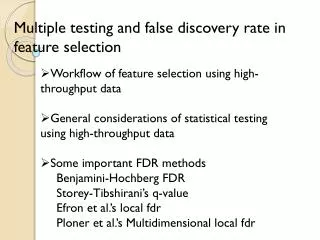
MAS 5.0 P/A Calls • Now based onWilcoxon’s one-sided signed rank test • Take differences between PM and MM (16 differences) • Rank the absolute differences from smallest to largest (1-16). Sign the ranks based on if differences were +/-. • If no differences expect sum of positive ranks to be about sum of negative ranks. (about 64 e.g., 1+3+5+7+9+11+13+15) • If really different then expect sum of negative ranks to be close to 0 or 1. • P-value (from table) of seeing smaller sum of ranks used to make calls. • P < 0.04 • 0.04 >= M <= 0.06 • A > 0.06 • Note: Making about 12,000 such calls per chip. • The probability of making a false present call is 0.05 for the test on a single gene but with12,000 tests there will be 600 spurious calls just by chance! • Multiple testing correction issue
Multiple Testing Correction • Family-wise Error Rate (FWER) • Control the probability of making any false positive call at the desired significance level. • Conservative methods such as the Bonferroni correction • Divide p-value by number of calls (or genes) • For 12,000 genes, need a p-value threshold of about 0.000004 for each gene to assure that the probability of making any false present call is 0.05 • False Discovery Rate (FDR) • FDR = expected (# false predictions/ # total predictions) • Control the proportion of false positive calls in all positive calls at the desired significance level. • Shifts focus to predicted positives and accepts that some will be wrong. An FDR of 0.05 means out of 100 predicted positives, 5 are wrong. • FWER will be very high but not important.
Benjamini-Hochberg FDR • Step-up method (sort p-values in decreasing order and evaluate until first success meeting cut-off) • http:// www.math.tau.ac.il/~ybenja/ • Cut-off of 0.02 FDR (only 2 expected false positives in 100 predictions) • For A chip (mostly known genes), this meant a cutoff of around 0.005 • 3000 to 4000 genes pass as expressed • 60 to 80 of these are wrong (i.e., about 0.005 of 12,000) • FDR chosen to maximize the number of genes passing the cutoff yet keeping the number of false calls small.
Results of Absolute Expression Analysis Table 1. Number of genes expressed in each population from bone marrow Table 2. Number of genes expressed in each population from fetal liver
Results of Absolute Expression Analysis (cont.) Table 3. Number of genes uniquely expressed in each population from bone marrow Table 4. Number of genes uniquely expressed in each population from fetal liver
2 Differential Expression Analysis Bone Marrow Sample LT-HSC ST-HSC LCP MBC analysis analysis analysis FetalLiverSample Our goal is to identify genes differentially expressed between HSCs and successive populations and to know the degree of confidence in the results. HSC LCP MBC analysis analysis
MAS 5.0 MAS 5.0 Gene1 e1(1) e1(2) e1(3) e1(4) Gene2 e2(1) e2(2) e2(3) e2(4) . . . GeneN eN(1) eN(2) eN(3) eN(4) Gene1 e1(1) e1(2) e1(3) e1(4) Gene2 e2(1) e2(2) e2(3) e2(4) . . . GeneN eN(1) eN(2) eN(3) eN(4) SAM LPE + BH PaGE Differential Expression Analysis LT-HSC ST-HSC Gene list 2 Gene list 3 Gene list 1 (Intersect) Final Gene list
MAS 5.0 Expression Level Estimate • Goals were to replace AvgDiff with a metric that produces only positive values and is little affected by outliers. • Tukey’s biweight and imputation of stray signal • Substitute negative PM-MM values with predicted values based on other probe pairs. • Instead of straight average, use average of values weighted by distance from median. (Can do iteratively but just do one step.) • Those furthest from the median contribute the least to the average.
Differential Expression Methods Used • PaGE (Pattern of Gene Expression) http://www.cbil.upenn.edu/PaGE/ • SAM (Significance Analysis of Microarrays) http://www-stat.stanford.edu/~tibs/SAM/index.html • LPE (Local Pooled-Error model test) http://hesweb1.med.virginia.edu/bioinformatics/
FDR Using Permutations • An alternative to the B-H FDR is to use a permutation method. • A single gene statistic is chosen • for PaGE it is simply the ratio of expression levels • for SAM it is a variant of the t-statistic. • The experiments are permuted between the groups and a permutation estimate of the null distribution of the statistic is compiled. • This distribution is then used to estimate what cutoff value for the single gene p-values will achieve the desired FDR based on the number of genes expected to pass the cut-off by chance and the observed number of genes that pass the cut-off. Permuted Observed
Using Permutations to Get p-values • Permutations randomize associations • use these associations to recalculate statistics for each permutation • Find the likelihood of the observed statistic based on the distribution of statistics from the permuted samples • p-value = percent of statistics generated from the permutations that are greater than or equal to the observed statistic. • Permuting columns preserves any gene dependencies but scrambles samples LT-HSC ST-HSC a b c d e f g h LT-HSC ST-HSC c d e f a b g h Permute columns to c,d,e,f;a,b,g,h
Example of Permutation for Eight Samples in Two Groups (4, 4) • Step 1: permute the sample columns (e.g., swap sample a in group 1 with the sample e in group 2). Calculate the t-statistic. Note: permuting columns avoids assumption of gene independence. Important for considering more than one gene. • Step 2: repeat step 1 for all possible permutations (70 in this case). • Step 3: Use the 70 t-statistics to get the distribution. • Step 4: compare starting t-statistic to distribution to get p-value (fraction of permuted t-statistics larger than observed t-statistic d) Permuted
Generating Permutations • 4, 4 (a,b,c,d;e,f,g,h) gives 70 permutations • No swap: a,b,c,d;e,f,g,h 1 • swap 1: b,c,d,e;a,f,g,h a,c,d,e;b,f,g,h a,b,d,e;c,f,g,h a,b,c,e;d,f,g,h 16 b,c,d,f;a,e,g,h etc… b,c,d,g;a,e,f,h etc… b,c,d,h;a,e,f,g etc… • swap 2: c,d,e,f;a,b,g,h b,d,e,f;a,c,g,h b,c,e,f;a,d,g,h a,d,e,f;b,c,g,h a,c,e,f;b,d,g,h a,b,e,f;c,d,g,h 36 c,d,e,g;a,b,f,h etc… c,d,e,h;a,b,f,g etc… c,d,f,g;a,b,e,h etc… c,d,f,h;a,b,e,g etc… c,d,g,h;a,b,e,f etc… • swap 3: d,e,f,g;a,b,c,h c,e,f,g;a,b,d,h b,e,f,g;a,c,d,h a,e,f,g;b,c,d,h 16 d,e,f,h;a,b,c,g etc… d,e,g,h;a,b,c,f etc… d,f,g,h;a,b,c,e etc… • swap 4: e,f,g,h;a,b,c,d 1
SAM confidence • SAM stands for “Statistical Analysis of Microarrays.” Tusher et al PNAS 2001. • SAM controls the FDR. • Note: A p-value of .05 is considered marginal. But a false-discovery rate as high as .50 might even be desirable. • SAM uses a variant of the t-statistic • Has a fudge factor s0 (a small positive constant) to limit the effect of high variation at low intensities. d(g) = x1(g) - x2(g) where s(g) = standard error for gene g s(g) + s0
PaGE • PaGE stands for Patterns from Gene Expression. • Goal is to compare patterns across more than 2 groups to look at co-regulation. • t-statistics not really applicable to describing co-regulation • PaGE was developed by our group at Penn! • Manduchi et al. Bioinformatics 2000. • PaGE also focuses on the FDR. • PaGE takes a minimum confidence level as a parameter, and finds all genes which exceed this confidence. • Each gene is reported with its own confidence. FDR = 1- Confidence • PaGE uses ratios of means. B , C , D A A A Where A, B, C, and D are group means for each gene and A is the reference group. • Use permutations to generate the random distribution of ratios.
Local Pooled Error • Uses the z-test • z = (median1 - median2)/spooled • Use medians instead of means • Variance from pools of genes • Pool genes to combine variance in signals • Divide genes up into quantiles (e.g. percentiles) based on average (log) expression value over replicated arrays and estimate variance for genes within each quantile. • Use local pooled variance for each gene comparison. With few replicates, this provides a better estimate of true variance in measurement. • Assuming normal distribution, use z-test to get p-values • Determine significance using multiple testing correction (B-H FDR).
MAS 5.0 MAS 5.0 Gene1 e1(1) e1(2) e1(3) e1(4) Gene2 e2(1) e2(2) e2(3) e2(4) . . . GeneN eN(1) eN(2) eN(3) eN(4) Gene1 e1(1) e1(2) e1(3) e1(4) Gene2 e2(1) e2(2) e2(3) e2(4) . . . GeneN eN(1) eN(2) eN(3) eN(4) SAM LPE + BH PaGE Differential Expression Analysis HSC LCP Gene list 2 Gene list 3 Gene list 1 (Intersect) Final Gene list
Results of Differential Expression Analysis • Bone Marrow Sample • LT-HSC vs. STHSC: 13 up-regulated in LT-HSC, 73 up-regulated in ST-HSC • ST-HSC vs. LCP: 25 up-regulated in ST-HSC, 28 up-regulated in LCP • LCP vs. MBC: 0 up-regulated in LCP, 219 up-regulated in MBC • Fetal Liver Sample • HSC vs. LCP: 9 up-regulated in HSC, 1 up-regulated in LCP • LCP vs. MBC: 108 up-regulated in LCP, 437 up-regulated in MBC
Comparison of current study with the original analysis in Ivanova et al., Science, 2002
More Information on Affymetrix • The 2003 Affymetrix GeneChip Microarray Low-Level Workshop • http://www.affymetrix.com/corporate/events/seminar/microarray_workshop.affx • Many slide presentations and posters available for download. • Bioconductor • http://www.bioconductor.org • Open source effort using the R statistical packages.
3 Cluster Analysis • Goal: look for genes with similar expression patterns across different hematopoietic populations. • Method: Self-Organizing Maps (SOM) • Distance measure: (1 – Pearson correlation coefficient) • Gene selection: analysis of variance (ANOVA) to select informative genes with significant expression level change across populations. Table: Number of genes selected for having significant expression level change over populations in different samples
Figure: Plot of expression profiles for genes in one cluster generated by SOM analysis for bone marrow sample. The centroid is indicated by the red line.