Download
1 / 28
280 likes | 395 Views
Accelerated Deployment of CO 2 Capture Technologies— ODT Simulation of Carbonate Precipitation. Review Meeting—University of Utah September 10, 2012. David Lignell and Derek Harris. Objectives. Year 2 Deliverables

E N D
Accelerated Deployment of CO2 Capture Technologies—ODT Simulation of Carbonate Precipitation Review Meeting—University of Utah September 10, 2012 David Lignell and Derek Harris
Objectives • Year 2 Deliverables • Validation study of ODT with acid/base chemistry and population balance against CO2 mineralization data identified in the scientific literature. • Quantification of relevant timescale regimes for mixing, nucleation, and growth processes with associated identification of errors in LES models. • Tasks • Implement acid/base chemistry and population balances in ODT code. • Identification studies for active timescales: turbulent mixing, nucleation, growth. • Quantification studies for influence of timescale approximations on particle sizes and polymorph selectivity. • Investigation of implications of timescales on LES models.
Progress • Focus on timescale analysis • Chemical Kinetic timescales • Mixing timescales in ODT • Ongoing kinetic development with Utah group • Heterogeneous nucleation • Coagulation • Beginning investigation of implications of timescales on LES models.
Basic Kinetic Processes • Mix two aqueous streams • Na2CO3, CaCl2 • Polymorphs: • ACC, Vaterite, Aragonite, Calcite • High super saturation ratio S causes precipitation • ACC nucleates quickly, reduces S to 1 • As other polymorphs nucleate and grow, ACC dissolves, maintaining S • When ACC is gone, S drops again, stepping through polymorphs. • Nucleation rates are key • Set ratios of number densities, which then grow/dissolve abundances ACC Nuc, Grw ACC Diss, Vat. Grw Key Dynamics occur– mixing dependence Vat Diss, ACC. Grw 80% precipitation in 1 s. Primarily ACC.
Basic Kinetic Processes • 80% precipitation • Occurs withing 1 s • Primarily ACC • No new particles after ~1 s.
Basic Kinetic Processes M3 M0 Moments VAT ACC Cal nuc grw Rates
Timescale Analysis • Goal • Quantify timescales: Reaction Mixing • Overlap of scales influences model development • Turbulent flows contain a range of scales. • Represented by the turbulent kinetic energy and scalar spectra. • Quantify large/small mixing scales: integral/Kolmogorov • Where are the reactions? • trxn > tmix no mixing model • trxn < tmix decoupled chemistry • trxn ≈ tmix T.C.I h LI
Approach Chemistry Mixing ODT idealized channel ODT homogeneous turbulence Energy Spectra Timescales • 0-D simulations • Matlab code • 4 polymorphs • Nucleation, Growth • Solve with DQMOM • Analyze QMOM rates
Kinetic Analysis • Timescales / Rates • Several approaches • ODE integration • Simple, global • Direct rates from system • Scaled nucleation and growth rates. • Jacobian matrix • Components • Eigenvalues • Other approaches
Kinetic Analysis Solving with explicit Euler. All Matlab solvers failed (long run times, or no solution). Stable timesteps for Adjusting stepsize as Verified accuracy by comparison of coefficient 0.1, 0.01. • Timescales / Rates • Several approaches • ODE integration • Simple, global • Direct rates from system • Scaled nucleation and growth rates. • Jacobian matrix • Components • Eigenvalues • Other approaches
Kinetic Analysis • Timescales / Rates • Several approaches • ODE integration • Simple, global • Direct rates from system • Scaled nucleation and growth rates. • Jacobian matrix • Components • Eigenvalues • Other approaches 0 “Timescales” range from 1E-11 seconds to 1 second, during a 1 second simulation.
Kinetic Analysis Lin and Segel “Mathematics applied to deterministic problems in the natural sciences” 1998. • Timescales / Rates • Several approaches • ODE integration • Simple, global • Direct rates from system • Scaled nucleation and growth rates. • Jacobian matrix • Components • Eigenvalues • Other approaches t
Direct Scales • Timescales / Rates • Several approaches • ODE integration • Simple, global • Direct rates from system • Scaled nucleation and growth rates. • Jacobian matrix • Components • Eigenvalues • Other approaches
Timescales from Eigenvalues 1-D Eigenvalues of Jacobian of RHS function are intrinsic rates, or inverse timescales. • Timescales / Rates • Several approaches • ODE integration • Simple, global • Direct rates from system • Scaled nucleation and growth rates. • Jacobian matrix • Components • Eigenvalues • Other approaches Multi-D
Timescales from Eigenvalues Linear t to 0.01 s • Sawada compositions • Timescale range • 1.2 ms to O(>1000 s) • Initial period is one of nucleation of particles. • Variations as growth processes activate at times 10-8-10-5 s. • Eigenvalue functions don’t preserve identities • sorting (“color jumping”) • Fast dynamics occur up front: t < 0.01 for t < 0.1 Log t to 10000 s
Vary Supersaturation Ratio Sawada • Vary the range of supersaturation ratios. • 1-10x Sawada. • Rates increase by (x100) • Dynamics occur faster, at earlier times. 10*SSawada
Vary Temperature 25 oC • Vary temperature • 25 oC – 50 oC • Rates are somewhat higher at higher temperature (but not much). • Dynamics occur at similar times. 50 oC
Other • Diagonals of Jacobian are very similar to the eigenvalues. • Investigaged and implemented eigenvalue tracking analysis • Kabala et al. Nonlinear Analysis, Theory, Methods, and Applications, 5(4) p 337-340 1981. • To overcome sorting/identity problems, allowing mechanism investigation. • Sensitivity analysis, CMC approaches • PCA discussions with Alessandro • DQMOM scales • Coagulation considered. Very little changes (timescales). • Heterogeneous nucleation
Summary • Timescales can be tricky to compute and interpret • Wide range of scales • Will overlap with mixing scales 10-10 10-8 10-6 10-4 10-2 10-0 102 104 ODE integration Direct Nucleation M0 Direct Growth M3 V.A.C ACC Eigenvalues Peak Init t=1s
Mixing Scales • Mixer configuration—ODT • Sawada streams: m0/m1 = 0.4 • 1 inch Planar, temporal channel flow • Re = 40,000 • Transport elemental mass fractions • Sc = n/D varies 120-1300 (H+, CaOH+)
Mixing Scales • Mixer configuration—ODT • Sawada streams: m0/m1 = 0.4 • 1 inch Planar, temporal channel flow • Re = 40,000 • Transport elemental mass fractions • Sc = n/D varies 120-1300 (H+, CaOH+)
Mixing Scales Kolmogorov Integral Velocity Length Time h LI
Scalar Mixing Sc > 1 gives fine structures at high wavenumbers Batchelor scale lf Mixing Scales Kolmogorov Integral Velocity Length Time
Mixing Scales Velocity Dissipation Rate • Channel flow config is in progress. • Challenging case • Non-homogeneous • Energy spectra windowing. • Full domain has a wide range of scales in channel flow • Velocity and scalar dissipation is noisy (128 rlz). • Both decay in time, but velocity decays towards a stationary value. Velocity RMS Scalar RMS Scalar Dissipation Rate
Mixing Scales Integral Scalar tu, tf (s) Velocity Kolmogrov, Batchelor Time(s) Scalar th, tl (s) Velocity Time(s)
Homogeneous Turbulence • Homogeneous turbulence simulations performed • Faster turnaround, analysis. • Initialize using Pope’s model spectrum • Scalar transport with Sc=850 (the avg) • Scalar initialized with scaled velocity field at Sawada average streams with peak mixf at 1. • u’ = 0.3 (channel at 0.005 seconds, peak value) • Li = 0.01 (~half channel); Ldom = 10Li Rel = 206 • Velocity decays, scalar pushes to high wavenumbers t=0.001 s t=0.02 s
Summary u Mixing—Integral MIXING f • Mixing and reaction scales overlap Mixing—Kolm./Batch f u 10-10 10-8 10-6 10-4 10-2 10-0 102 104 ODE integration Direct Nucleation M0 REACTION Direct Growth M3 V.A.C ACC Eigenvalues Peak Init t=1 s
Summary • Wide range in reaction timescales • Mixing and reaction timescales are not widely disparate • Test homogeneous mixing, vary mixing rates. • LES model implications and testing