Regional Arctic Climate System Model (RACM) – Project Overview

1. Regional Arctic Climate System Model (RACM) – Project Overview A 4-year (2007-2010) DOE / SciDAC-CCPP project Participants: Wieslaw Maslowski (PI) - Naval Postgraduate School John Cassano (co-PI) - University of Colorado William Gutowski (co-PI) - Iowa State University Dennis Lettenmeier (co-PI) - University of Washington Greg Newby, Andrew Roberts, - Arctic Region Supercomputing Juanxiang He, Anton Kulchitsky Center Dave Bromwich and Keith Hines (OSU), Gabriele Jost (HPCMO), Tony Craig (NCAR), Jaromir Jakacki (IOPAN), Mark Seefeldt (CU), Chenmei Zhu (UW), Justin Glisan Brandon Fisel (ISU), Jaclyn Kinney (NPS) IARC / Arctic System Model Workshop, Boulder, CO, May 19-21, 2008

2. Main science objective Specific Goals To synthesize understanding of past and present states and thus improve decadal to centennial prediction of future Arctic climate and its influence on global climate. • develop a state-of-the-art Regional Arctic Climate system Model (RACM) including high-resolution atmosphere, ocean, sea ice, and land hydrology components • perform multi-decadal numerical experiments using high performance computers to understand feedbacks, minimize uncertainties, and fundamentally improve predictions of climate change in the pan-Arctic region • provide guidance to field observations and to GCMs on required improvements of future climate change simulations in the Arctic

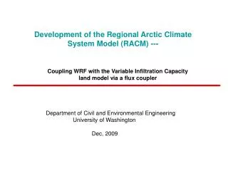
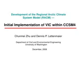
3. Regional Arctic climate modelcomponents and resolution • Atmosphere - Polar WRF(gridcell ≤50km) • Land Hydrology – VIC (gridcell ≤50km) • Sea Ice – CICE/CSIM(gridcell ≤10km) • Ocean - POP(gridcell ≤10km) • Flux Coupler – CCSM/CPL7

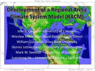
4. (red box represents the domain of ocean and sea ice models) RACM domain and elevations • Pan-Arctic region to include: • all sea ice covered ocean in the northern hemisphere • Arctic river drainage • critical inter-ocean exchange and transport • large-scale atmospheric weather patterns (AO, NAO, PDO)

5. Why develop a regional Arctic climate model? • Facilitate focused regional studies of the Arctic • Resolve critical details of land elevation, coastline and ocean bottom bathymetry • Improve representation of local physical processes and feedbacks (e.g. forcing and deformation of sea ice) • Minimize uncertainties and improve predictions of climate change in the pan-Arctic region

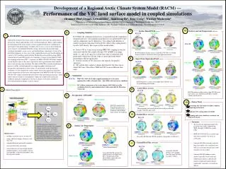
6. Comparison of sea ice conditions in September 2002 Arctic Sea Ice cover in September 2002 3 3 3 2 2 2 1 1 1 CCSM3(b) simulates too much ice on the Greenland shelf (1), too much/little melt in the eastern(2) / western(3) Arctic. NCAR/CCSM3 case (b30.040b) prediction of summer ice-free Arctic by 2050

7. Comparison of areal sea ice fluxes through Fram Strait • CCSM3 sea ice export about twice as high as compared to • Kwok et al. (2003) and NPS/NAME fluxes • Possibly too strong atmospheric forcing at Fram Strait • Consequences include • too much ice production in the Arctic Ocean • overestimate of buoyancy flux into the North Atlantic

8. 25-year mean ocean volume transport (Sv) / heat transport (TW) Note: 1Sv = 10 m6/sec; 1TW = 3.6 Petajoules/hour or 86.4 Petajoules/day or 2592 Petajoules/month NPS/NAME TRANSPORTS (Maslowski et al., JGR, 2004) Fram Strait ‘in’ obs estimates: 7.0 Sv / 50 TW - Courtesy of A. Beszczynska-Möller, AWI FJL-NZ: near-zero heat transport (Gammelsrod et al., JMS submitted)

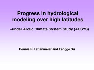
9. OCEAN BATHYMETRY/RESOLUTION IMPACTS 18-km Model 0-225 m (levels 1-7), every vector 9-km Model 0-223 m (levels 1-15), every 2nd vector • Barents Sea outflows (north of Novaya Zemlya and through Kara Gate) look similar but: • Mean paths significantly different due to representation of bathymetry (I.e. resolution) • Velocity magnitudes differences • 9-km model circulation shown to match observed well (Maslowski et al., 2004) • Implications for location of fronts, water mass transformations, heat and salt balances • (from Maslowski et al., 2008)

10. LAND TOPOGRAPHY / RESOLUTION IMPACTS ERA40 Annual Precipitation ERA40 Annual Precipitation • Increased horizontal resolution allows for improved representation of topography • Topography impacts atmospheric circulation, precipitation, temperature, etc. Polar MM5 Annual Precipitation • ERA40 precipitation (above) is “smoothed” compared to higher resolution (50 km) Polar MM5 simulation (right) • This will impact both atmosphere and land/ocean

11. Cyclone Central Pressure and Size • Model resolution impacts the size and intensity of cyclones • Comparison of AMPS ( 20 km; based on Polar MM5 and WRF) and three coarser reanalyses in the Southern Ocean • AMPS simulates lower pressure in and smaller cyclones than all reanalyses • Similar results are expected in Arctic

12. Finer resolution captures dispersed features missed by coarse grids RMS Difference vs. Baseline (500 hPa Heights) Wetlands cases Unforced “noise” Wetlands Gutowski et al. (2007)

13. Attribution of observed trends in Eurasian Arctic river runoff: Why don’t model reconstructed trends match observations? • Long-term streamflow changes (Peterson et al., 2002) are not captured by model in permafrost basins (particularly in discontinuous permafrost). • Reasons include improper permanent ground ice initialization and lack of tracking. High Quality GHCN Precipitation Stations • Improvements to the VIC frozen soils algorithm to handle permafrost are underway. High Quality GHCN Temperature Stations (Visuals courtesy of Jennifer Adam, Washington State University)

14. Sea Ice Divergence near SHEBA Tower (Stern & Moritz, 2002) Ice strain (reds/yellows) (200km x 200 km)

15. RACM 2008-2009 Outlook • Evaluate uncoupled model simulations for physical and numerical optimizations in RACM • Couple each climate model component to the coupler (CPL7) • Run and validate results as in #2 • Couple all climate model components and run tests with RACM

16. Movie of Daily Sea Ice Divergence