Download
1 / 47
480 likes | 499 Views
The Capital Asset Pricing Model (Chapter 8). Premise of the CAPM Assumptions of the CAPM Utility Functions The CAPM With Unlimited Borrowing and Lending at a Risk-Free Rate of Return

E N D
The Capital Asset Pricing Model (Chapter 8) • Premise of the CAPM • Assumptions of the CAPM • Utility Functions • The CAPM With Unlimited Borrowing and Lending at a Risk-Free Rate of Return • Capital Market Line Versus Security Market Line • Relationship Between the SML and the Characteristic Line • The CAPM With No Risk-Free Asset • The CAPM With Lending at the Risk-Free Rate, but No Borrowing • The CAPM With Lending at the Risk-Free Rate, and Borrowing at a Higher Rate • Market Efficiency
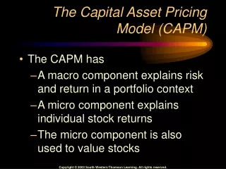
Premise of the CAPM • The Capital Asset Pricing Model (CAPM) is a model to explain why capital assets are priced the way they are. • The CAPM was based on the supposition that all investors employ Markowitz Portfolio Theory to find the portfolios in the efficient set. Then, based on individual risk aversion, each of them invests in one of the portfolios in the efficient set. • Note, that if this supposition is correct, the Market Portfolio would be efficient because it is the aggregate of all portfolios. Recall Property I - If we combine two or more portfolios on the minimum variance set, we get another portfolio on the minimum variance set.
One Major Assumption of the CAPM • Investors can choose between portfolios on the basis of expected return and variance. This assumption is valid if either: • 1. The probability distributions for portfolio returns are all normally distributed, or • 2. Investors’ utility functions are all in quadratic form. • If data is normally distributed, only two parameters are relevant: expected return and variance. There is nothing else to look at even if you wanted to. • If utility functions are quadratic, you only want to look at expected return and variance, even if other parameters exist.
Evidence Concerning Normal Distributions • Returns on individual stocks may be “fairly” normally distributed using monthly returns. For yearly returns, however, distributions of returns tend to be skewed to the right. (-100% is the largest possible loss; upside gains are theoretically unlimited, however. • Returns on portfolios may be normally distributed even if returns on individual stocks are skewed.
Utility Functions • Utility is a measure of well-being. • A utility function shows the relationship between utility and return (or wealth) when the returns are risk-free. • Risk-Neutral Utility Functions: Investors are indifferent to risk. They only analyze return when making investment decisions. • Risk-Loving Utility Functions: For any given rate of return, investors prefer more risk. • Risk-Averse Utility Functions: For any given rate of return, investors prefer less risk.
Utility Functions (Continued) • To illustrate the different types of utility functions, we will analyze the following risky investment for three different investors:
Risk-Neutral Investor • Assume the following linear utility function: ui = 10ri
Risk-Neutral Investor (Continued) • Expected Utility of the Risky Investment: • Note: The expected utility of the risky investment with an expected return of 30% (300) is equal to the utility associated with receiving 30% risk-free (300).
Risk-Neutral Utility Functionui = 10ri Total Utility Percent Return
Risk-Loving Investor • Assume the following quadratic utility function: ui = 0 + 5ri + .1ri2
Risk-Loving Investor (Continued) • Expected Utility of the Risky Investment: • Note: The expected utility of the risky investment with an expected return of 30% (280) is greater than the utility associated with receiving 30% risk-free (240). • That is, the investor would be indifferent between receiving 33.5% risk-free and investing in a risky asset that has E(r) = 30% and (r) = 20%
Risk-Loving Utility Functionui = 0 + 5ri + .1ri2 Total Utility 500 280 240 60 10 30 33.5 50 Percent Return
Risk-Averse Investor • Assume the following quadratic utility function: ui = 0 + 20ri - .2ri2
Risk-Averse Investor (Continued) • Expected Utility of the Risky Investment: • Note: The expected utility of the risky investment with an expected return of 30% (340) is less than the utility associated with receiving 30% risk-free (420). • That is, the investor would be indifferent between receiving 21.7% risk-free and investing in a risky asset that has E(r) = 30% and (r) = 20%.
Risk-Averse Utility Functionui = 0 + 20ri - .2ri2 Total Utility 500 420 340 180 10 21.7 30 50 Percent Return
Indifference Curve • Given the total utility function, an indifference curve can be generated for any given level of utility. First, for quadratic utility functions, the following equation for expected utility is derived in the text:
Indifference Curve (Continued) • Using the previous utility function for the risk-averse investor, (ui = 0 + 20ri - .2ri2), and a given level of utility of 180: • Therefore, the indifference curve would be:
Risk-Averse Indifference CurveWhen E(u) = 180, and ui = 0 + 20ri - .2ri2 Expected Return Standard Deviation of Returns
Maximizing Utility • Given the efficient set of investment possibilities and a “mass” of indifference curves, an investor would maximize his/her utility by finding the point of tangency between an indifference curve and the efficient set. Expected Return E(u) = 380 E(u) = 280 Portfolio That Maximizes Utility E(u) = 180 Standard Deviation of Returns
Problems With Quadratic Utility Functions • Quadratic utility functions turn down after they reach a certain level of return (or wealth). This aspect is obviously unrealistic: Total Utility Unrealistic Percent Return
Problems With Quadratic Utility Functions (Continued) • As discussed in the Appendix on utility functions, with a quadratic utility function, as your wealth level increases, your willingness to take on risk decreases (i.e., both absolute risk aversion [dollars you are willing to commit to risky investments] and relative risk aversion [% of wealth you are willing to commit to risky investments] increase with wealth levels). In general, however, rich people are more willing to take on risk than poor people. Therefore, other mathematical functions (e.g., logarithmic) may be more appropriate.
Two Additional Assumptions of the CAPM • Assumption II - All investors are in agreement regarding the planning horizon (i.e., all have the same holding period), and the distributions of security returns (i.e., perfect knowledge exists). • Assumption III - There are no frictions in the capital market (i.e., no taxes, no transaction costs, no restrictions on short-selling). • Note: Many of the assumptions are obviously unrealistic. Later, we will evaluate the consequences of relaxing some of these assumptions. The assumptions are made in order to generate a model that examines the relationship between risk and expected return holding many other factors constant.
The CAPM With Unlimited Borrowing & Lending at a Risk-Free Rate of Return • First, using the Markowitz full covariance model we need to generate an efficient set based on all risky assets in the universe: Expected Return Standard Deviation of Returns
Capital Market Line (CML) • Next, the risk-free asset is introduced. The Capital Market Line (CML) is then determined by plotting a line that goes through the risk-free rate of return, and is tangent to the Markowitz efficient set. This point of tangency identifies the Market Portfolio (M). The CML equation is:
Capital Market Line (CML) - Continued Expected Return Borrowing CML Lending M E(rM) rF (rM) Standard Deviation of Returns
Portfolio Risk and the CML • Note that all points on the CML except the Market Portfolio dominate all points on the Markowitz efficient set (i.e., provide a higher expected return for any given level of risk). Therefore, all investors should invest in the same risky portfolio (M), and then lend or borrow at the risk-free rate depending on their risk preferences. • That is, all portfolios on the CML are some combination of two assets: (1) the risk-free asset, and (2) the Market Portfolio. Therefore, for portfolios on the CML:
Portfolio Risk and the CML (Continued) • By definition, since (rp) = xM(rM), all portfolios that lie on the CML are perfectly positively correlated with the Market Portfolio (i.e., 100% of the variance in the portfolio’s returns is explained by the variance in the market’s returns, when the portfolio lies on the CML). • Recall the Single-Factor Model’s Measure of Variance Note, since (rM) is the same for all portfolios, all of the risk of a portfolio on the CML is reflected in its beta.
Capital Market Line (CMLVersusSecurity Market Line (SML) • Recall Property II: Given a population of securities, there will be a simple linear relationship between the beta factors of different securities and their expected (or average) returns if and only if the betas are computed using a minimum variance market index portfolio. • Therefore: Given the CML, we can determine the SML (relationship between beta & expected return)
CML Versus SML E(r) E(r) CML C SML M C M E(rM) E(rM) B B A A rF rF (r) (rM)
Portfolios That Lie on the CMLWill Also Lie on the SML • CML Equation: • Can be restated as: • And, since for portfolios on the CML: • We can state that for portfolios on the CML:
Therefore, for portfolios on the CML: Individual Securities Will Lie on the SML, But Off the CML Recall: However: in well diversified portfolios (i.e., can be done away with)
Therefore,Relevant Risk may be defined as: And since: We can state that: That is, a security’s contribution to the risk of a portfolio can be measured by its beta. Since an individual security’s residual variance can be diversified away in a portfolio, the market place will not reward this “unnecessary” risk. Since only beta is relevant, individual securities will be priced to lie on the SML.
Individual Security on the SML and Off the CML (Continued) E(r) E(r) CML SML 22 22 M M 18 18 Off the CML On the SML 10 10 (r) 22.5 33.75 1.5
Relationship Between the SML and the Characteristic Line (In Equilibrium) • Characteristic Line: • Security Market Line (SML): • As a result, in equilibrium, all characteristic lines “pass through” the risk-free rate.
Characteristic Line Versus SML(In Equilibrium) rj E(r) A1 = 10(1 - .5) = 5 A2 = 10(1 - 1.5) = -5 E(r2) E(r2) E(rM) E(rM) 2 = 1.5 E(r1) E(r1) rF rF 1 =.5 A1 rM E(rM) = A2 Characteristic Line Security Market Line
Characteristic Line Versus SML (In Disequilibrium: Undervalued Security) rj E(r) E(r2) E(r2) E(rE) E(rE) 2 = 1.5 E(rM) E(rM) rF rF rM E(rM) = AE Characteristic Line Security Market Line
Characteristic Line Versus SML (In Disequilibrium: Overvalued Security) E(r) rj E(rE) E(rE) E(r2) E(rM) 2 = 1.5 E(r2) rF rF rM E(rM) = AE Characteristic Line Security Market Line
CAPM With No Risk-Free Asset E(r) E(r) SML E(rM) X M E(rM) E(rZ) MVP E(rZ) (r)
CAPM With No Risk-Free Asset (Continued) • Assumption: All investors take positions on the efficient set (Between MVP and X) • In this case, the Markowitz efficient set (MVP to X) is the Capital Market Line (CML). • M is the efficient Market Portfolio (the aggregate of all portfolios held by investors) • E(rZ) is the intercept of a line drawn tangent to (M) • From Property II, since (M) is efficient, a linear relationship exists between expected return and beta. All assets (efficient and inefficient) will be priced to lie on the SML.
Can Lend, but Cannot Borrow at the Risk-Free Rate E(r) E(r) SML X E(rM) E(rM) M L E(rZ) E(rZ) rF (r) (rM)
Can Lend, but Cannot Borrow at the Risk-Free Rate (Continued) • Capital Market Line (CML): • (rF - L - M - X) • Between rF and L: • Combinations of the risk-free asset and the risky (efficient) portfolio L. • Between L and X: • Risky portfolios of assets. • Security Market Line (SML): • All assets (efficient and inefficient) will be priced to lie on the SML.
Can Lend at the Risk-Free Rate:Borrowing is at a Higher Rate E(r) E(r) X SML B E(rM) E(rM) M rB L E(rZ) E(rZ) rF (r) (rM)
Can Lend at the Risk-Free Rate, and Borrow at a Higher Rate (Continued) • Capital Market Line (CML): • (rF - L - M - B - X) • Between rF and L: • Combinations of the risk-free asset and the risky (efficient) portfolio L. • Between L and B: • Risky portfolios of assets. • Between B and X: • Combinations of the risky (efficient) portfolio B and a loan with an interest rate of rB • Security Market Line (SML): • All assets (efficient and inefficient) will be priced to lie on the SML
Conditions Required for Market Efficiency • In order for the Market Portfolio to lie on the efficient set, the following assumptions must hold: • All investors must agree about the risk and expected return for all securities. • All investors can short-sell all securities without restriction. • No investor’s return is exposed to federal or state income tax liability now in effect. • The investment opportunity set of securities is the same for all investors.
When the Market Portfolio is Inefficient • Investors Disagree About Risk and Expected Return • In this case there will be no unique perceived efficient set for the Market Portfolio to lie on (i.e., different investors would have different perceived efficient sets). • Some Investors Cannot Sell Short • In this case, Property I no longer holds. If a “constrained” efficient set were constructed with no short-selling, and each investor selected a portfolio lying on the “constrained” efficient set, the combination of these portfolios would not lie on the “constrained” efficient set.
When the Market Portfolio is Inefficient (Continued) • Taxes Differ Among Investors • When tax exposure differs among investors (e.g., state, local, foreign, corporate versus personal), the after-tax efficient set for one investor will be different from that of others. There would be no unique efficient set for the Market Portfolio to lie on. • Alternative Investments Differ Among Investors • Efficient sets will differ among investors when the populations of securities used to construct the efficient sets differ (e.g., some may exclude polluters, others may include foreign assets, etc.).
Summary of Market Portfolio Efficiency • In reality, assumptions underlying the efficiency of the Market Portfolio are frequently violated. Therefore, the Market Portfolio may well lie inside the efficient set even if the efficient set is constructed using the population of securities making up the market. In other words, perhaps the market can be beaten. That is, there may be portfolios that offer higher risk-adjusted returns than the overall Market Portfolio.