Download
1 / 23
250 likes | 356 Views
Extreme Value Theory for High Frequency Financial Data. Abhinay Sawant April 20, 2009 Economics 201FS. Background: Value at Risk.

E N D
Extreme Value Theory for High Frequency Financial Data Abhinay Sawant April 20, 2009 Economics 201FS
Background: Value at Risk • An important topic in financial risk management is the measurement of Value at Risk (VAR). For example, if the 10-Day VAR of a $10 million portfolio is estimated to be $1 million, then we would interpret this is as: “We are 99% certain that we will not lose more than $1 million in the next 10 days.” • VAR is typically used as a gauge of exposure to financial risk for firms and regulators to determine the amount of capital to set aside to cover unexpected losses. VAR is also used to set risk limits by firms on individual traders. • Although practitioners typically calculate VAR based on the normal distribution, experience has shown that asset returns have fatter tails and asymmetry in tail distributions. An alternative approach that takes these issues into consideration is Extreme Value Theory.
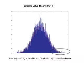
Background: Extreme Value Theory • Under order statistics, one normally imagines that the distribution of the maximum return max{r1, …, rn} converges to either 0 or 1: • Given independent and identically distributed log returns {r1, …, rn} the maximum follows the Generalized Extreme ValueDistribution:
Motivation: High-Frequency Data • There is limited literature on the use of the high-frequency data for Extreme Value Theory VAR estimation. This paper aims to implement EVT with actual stock price data and realize the benefits of using data at high-frequency. • Potential Benefits to high-frequency data is: • Better Estimation: More high-frequency returns allow for better chance of getting extreme returns. • Intraday VAR: Rather than setting aside capital once a day, adjusting the VAR depending on time of day may minimize capital. • Use of Recent Data: Some EVT methods such as Block Maxima require large amounts of data. High-frequency data allows more financial data from more recent years.
Methods: Block Maxima Estimation • Divide the time series {r1, …, rn} into blocks of size n and pull out the maximum of each block: {r1, …, rn} {r1, …, rn} {r1, …, rn} … • Use the maximums of each block to estimate the parameters of the GEV distribution (maximum likelihood). • In order to determine the value at risk:
Methods: Standardization of Data • One of the assumptions behind GEV estimation is that the data is independent and identically distributed. In order to meet this assumption, we divide the log return by the realized variance (measured by high-frequency and sampling) over the same time period: Half-Day Return RV (10 min) One-Day Return RV (10 min) Half-Day Return RV (10 min)
Methods: Predicting VAR • GEV distribution is fitted to standardized data, and VAR is determined in standardized terms. The VAR in real terms is then determined by un-standardizing the data by multiplying by tomorrow’s realized volatility: • Tomorrow’s realized volatility is either: • Known: Tests the validity of the extreme value distribution for VAR. • Forecasted: Using HAR-RV regression:
Methods: Testing the VAR Model • Binomial Distribution: Given a VAR model with probability p of exceedance of n trials, then the number of exceedances should be binomially distributed as Bin(n,p). Therefore, a p-value is calculated for a two-sided test exceedances compared to expected value np. • Kupiec Statistic: The p-value for a powerful two-tailed test proposed by Kupiec is also calculated. m = exceedances p = probability of exceedance n = trials
Model: Testing the VAR Model • Bunching: The following is the test statistic proposed by Christofferson. A low p-value suggests bunching is likely. • Mean VAR: Since the level of VAR sets the level of capital allocated for unexpected loss, a good VAR test would minimize the amount of capital allocated.
Results: EVT from 1-Day Returns(1912 Trials, Known Future RV) Left Tail Right Tail
Results: EVT from 1-Day Returns(1912 Trials, Forecasted RV) Left Tail Right Tail
Results: Intraday VAR(Known Future RV, Right Tail, 0.5% VAR)
Conclusions • Given sufficient knowledge about future realized volatility, extreme value theory appears to provide a good measurement of VAR. • Volatility forecasting problems appear to cause more issues with the left tail than the right. • Given sufficient knowledge about future realized volatility, intraday VAR seems plausible and a good method to minimize the use of capital.
Final Computations • Forecasting daily VAR from intraday VAR using the horizon rule: • Realized volatility forecasting for intraday volatility • Testing the other two EVT methods: (1) Peaks Over Thresholds, (2) Nonparametric Hill Estimation