Download
1 / 53
570 likes | 860 Views
Synchrotron radiation: generation, coherence properties and applications for beam diagnostics Gianluca Geloni European XFEL GmbH. Caveats, Acknowledgments and References. My experience with SR was mainly focused on e- beams and undulators Some articles/notes I co-authored on the subject:

E N D
Synchrotron radiation: generation, coherence properties and applications for beam diagnostics GianlucaGeloni European XFEL GmbH
Caveats, Acknowledgments and References • My experience with SR was mainly focused on e- beams and undulators • Some articles/notes I co-authored on the subject: • ‘Paraxial Green’s function in SR theory’, DESY 05-032, G. Geloni, E. Saldin, E. Schneidmiller and M. Yurkov http://arxiv.org/abs/physics/0502120 • A study on ‘Transverse coherence properties of X-ray beams in third-generation synchrotron radiation sources’ can be found in G. Geloni, E. Saldin, E. Schneidmiller and M. Yurkov NIM A 588 (2008) 463 • Fourier treatment of near-field synchrotron radiation theory, Gianluca Geloni, Evgeni Saldin, Evgeni Schneidmiller, Mikhail Yurkov, Optics Communications 276 (2007) 167–179 • I wish to thank E. Saldin for many discussions during the preparation of this talk
Contents Contents • Generation of radiation from a single charged particle • SR in general, approximations and characteristics • Example: BM radiation • Wavefront propagation • Coherence properties • Many particles, statistical optics treatment, coherence • Near and Far zone • SR and particle diagnostics (beam size measurements) • Application • Parameters for the CERN case of interest • Conclusions
Classical framework • From Maxwell eqs we arrive at the wave equations for E and B: • Use space-frequency representation • Use space-frequency representation to obtain the wave equations in the space-frequency domain: • Component by component: inhomogeneous Helmholtz Equation
Source & geometry specification • We first specialize to a single particle. We set the sources in the space-frequency as: x P r’(t’) z s=s(t’) is the curvilinear abscissa and we re-parametrizet’=t’(z); we assume constant speed. • We introduce y This can always be done. It is useful in the case when the field envelope is a slowly varying function of z wrtl
Green Function Solution for Helmholtz equation • For zo>z’ we can show that Here f0:time slippage photon-to-charge on the z axis in units of 1/w fr: difference of fly-time between photon from r’ to r0 and photon between z’ and z0 in units of 1/w
Formation Length • When the total phase varies of ~1, as we move along z’, the integrand begins to oscillate zero extra-contribution to the integral. • Let us first analyze Definition of formation length Lf: interval Dz’ such that Df0=1 • We now analyze the second phase term • At what condition we obtain variations, along Dz ~Lf , of a quantity ~1? • It can be demonstrated that sufficient condition is
Paraxial Approximation Whenever the paraxial approximation applies, i.e. when: (And additionally ) It can be shown that the total expression for the field boils down to
Ultrarelativistic Approximation • We now assume (always ok in our case) ultrarelativistic charges gz>>1 z • What can we say about the formation length Lf ? ~1 Since gz>>1 it follows Lf>>l/(2p) Condition to have variation in the second phase factor ~1 Implies automatically Ultrarelativistic approximation Paraxial approximation!
Ultrarelativistic Approximation and U.R. appr. applies Summing up. Whenever (Always in our case!) The formation length Lf >>l/(2p) Radiation is confined into a cone The paraxial approximation applies The field can be calculated as: Important note: for a single charge far zone simply means z0 >> Lf
Bending Magnet, single particle, far zone z0>>Lf And redefine z’ z’ + R qx ; then we have: For lc/(2p)~R/g3 • Lf~R/g, q~1/g Sometimes it is convenient to define
Bending Magnet, single particle, far zone z0>>Lf In those units, the above expression is equivalent to fx(rad) Ix(AU) x=1 fy(rad) Iy(AU)
Synchrotron Radiation Propagation We calculated the field at a given position z (does not matter where!) Then, we can calculate the field at any other position in free-space using We can even propagate at (virtual) positions actually occupied by sources!
Synchrotron Radiation Propagation Free-space propagation can be easily analyzed in the spatial Fourier domain Field propagation in the spatial Fourier domain is almost trivial. Note that the field can be seen as a superposition of plane waves angular spectrum u corresponds to a given propagation angle
Synchrotron Radiation Propagation We can start with the field distribution in the far zone, and calculate the field distribution at the ‘virtual’ source position, in the middle of the magnet! The field at z=0 is “virtual”. That particular field distribution at z=0 reproduces all effects associated with sources Note that free space basically acts as a Fourier Transform
Bending Magnet virtual source For a BM, the field seen by imaging the middle of the magnet (virtual source) with a lens is
Synchrotron Radiation Propagation Radiation from a single chargeis like a special (non-Gaussian) laser beam Rayleigh length Lf
SR and statistical optics Shot noise random position, direction, but also arrival time • Current fluctuations Random variables: e- angle + offset: Arrival times tk SR is a random process Statistical Optics! On top of that: energy spread, which I will not consider here… so, the full phase-space!
Simplifications Much largerrelative spectralwidth s=2.5e-10 s sw =1/s=4e9 Hz <<1
Relation with intensity and coherence Cross-spectral density and measured intensity Cross-spectral density and spectral degree of coherence Requirement on longitudinal coherence lc=l2/(Dl) >> max optical path difference
How to calculate G explicitly We need generalization of the field to account for offset and deflection of particles Call with y0 (virtual source) orexp[ip z q2/l]yf (far zone) any polarization component of the previously calculated fields and Introduce normalized units Virtual source Far zone
How to calculate G explicitly New variables: Cross-spectral density at the virtual source Cross-spectral density in the far zone
How to calculate G explicitly: models… Assume horizontal and vertical motions uncoupled Assume Gaussian particle beam shapes and divergences Assume min b-functions at the virtual source position (z=0)
Far zone for G Far zone definition For a single charge on axis: • Spherical wavefront For the cross spectral density we rely on a similar definition.
Overall General expression for G Cross-spectral density at the virtual source Cross-spectral density in the far zone
First asymptote: diffraction limit Suppose first Nx<<1, Ny<<1, Dx<<1, Dy<<1 Cross-spectral density at the virtual source Cross-spectral density in the far zone
Second asymptote: geometrical optics limit Now consider Nx>>1, Ny>>1, Dx>>1, Dy>>1 Cross-spectral density at the virtual source Cross-spectral density in the far zone
Second asymptote: geometrical optics limit Let’s have a closer look Nx>>1, Ny>>1, Dx>>1, Dy>>1 Cross-spectral density at the virtual source Cross-spectral density in the far zone
The VCZ theorem Let’s have a closer look Nx>>1, Ny>>1, Dx>>1, Dy>>1 Cross-spectral density at the virtual source I0 FT Cross-spectral density in the far zone gf
The VCZ theorem Let’s have a closer look Nx>>1, Ny>>1, Dx>>1, Dy>>1 Cross-spectral density at the virtual source I0 g0 FT FT Cross-spectral density in the far zone gf If
The VCZ theorem THIS IS JUST THE Van Cittert-Zernike Theorem (and its inverse, because near and far zone are reciprocal) Cross-spectral density at the virtual source I0 g0 FT FT Cross-spectral density in the far zone gf If
The VCZ theorem Van Cittert-Zernike Theorem r d S Van Cittert-Zernike theorem:For a QH stochastic process, power spectral density (intensity) on source, I0 and gf form a Fourier pair (Coherence length normalized to diffraction size!)
The VCZ theorem …we can even follow g as a function of z!
How do we treat other cases? Example: study case Nx>>1, Ny>>1, Dx<<1, Dy<<1 Cross-spectral density at the virtual source Cross-spectral density in the far zone
How do we treat other cases? Example: study case Nx>>1, Ny>>1, Dx<<1, Dy<<1 Cross-spectral density at the virtual source I0 Cross-spectral density in the far zone FT gf
Can we find the beam size? Different alternative methods (Nx>>1, Ny>>1, Dx<<1, Dy<<1): We can measure the intensity at the virtual source using a lens We can measure the fringe visibility in the far zone In principle we can even measure the fringe visibility at any position, but in this case we need a-priori information on the charged beam divergence in order to get back N… …remember:
Can we find the beam size? Going to Nx~1, Ny~1, Dx<<1, Dy<<1 we can still say something but analysis implies deconvolution: Virtual source Far zone
CERN parameter case How about our case? Moreover I took lmin = 200nm; lmax = 900nm
Formation length and critical wavelength Lf(m) lc[mm] g l g • Caveat: Whether there is enough light in the visible is another matter of concern, and should be considered separately.
Beam 1 – Main paramaters How about our case? Beam 1 Ny l Dy g l g
Beam 1 – main parameters How about our case? Beam 1 Far zone for ( z[m] )2 much larger than g l Y Note: for z=26 m, z2=676 m2
Beam 2 – main parameters How about our case? Beam 2 l Dy Ny g l g
Beam 2 – main parameters How about our case? Beam 2 Far zone for ( z[m] )2 much larger than g l Y Note: for z=26 m, z2=676 m2
Where can we use SR for diagnostics? • Challenging for N<<1, D<<1 • Still, there are “intermediate regions” where N>1, (with D<<1) • The reason for the existence of these “intermediate regions” ( even if e<<l/(2p) ), is that the beta are large