Download
1 / 25
270 likes | 472 Views
EEG/MEG source reconstruction. Jérémie Mattout / Christophe Phillips / Karl Friston. Wellcome Dept. of Imaging Neuroscience , Institute of Neurology, UCL, London. Estimating brain activity from scalp electromagnetic data. Sources. MEG data. Source Reconstruction.

E N D
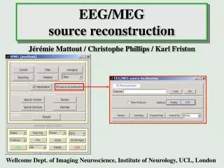
EEG/MEGsource reconstruction Jérémie Mattout / Christophe Phillips / Karl Friston Wellcome Dept. of Imaging Neuroscience, Institute of Neurology, UCL, London
Estimating brain activity from scalp electromagnetic data Sources MEG data Source Reconstruction ‘Equivalent Current Dipoles’ (ECD) ‘Imaging’ EEG data
Components of the source reconstruction process Source model ‘ECD’ ‘Imaging’ Forward model Registration Inverse method Data Anatomy
Components of the source reconstruction process Forward model Inverse solution Source model Registration
Source model Compute transformation T Individual MRI Templates Apply inverse transformation T-1 Individual mesh input functions output • Individual MRI • Template mesh • spatial normalization into MNI template • inverted transformation applied to the template mesh • individual mesh
fiducials fiducials Rigid transformation (R,t) Individual sensor space Individual MRI space Registration input functions output • sensor locations • fiducial locations • (in both sensor & MRI space) • individual MRI • registration of the EEG/MEG data into individual MRI space • registrated data • rigid transformation
Model of the head tissue properties Individual MRI space Foward model p Compute for each dipole + K n Forward operator functions input output • single sphere • three spheres • overlapping spheres • realistic spheres • sensor locations • individual mesh • forward operator K BrainStorm
1 dipole source per location Y = KJ+ E [nxt] [nxt] [nxp] [pxt] : min( ||Y – KJ||2 + λf(J) ) J J Inverse solution (1) - General principles General Linear Model Cortical mesh n : number of sensors p : number of dipoles t : number of time samples Under-determined GLM ^ Regularized solution data fit priors
E1 ~ N(0,Ce) Y = KJ + E1 E2 ~ N(0,Cp) J = 0 + E2 Ce = 1.Qe1 + … + q.Qeq Cp = λ1.Qp1 + … + λk.Qpk Inverse solution (2) - Parametric empirical Bayes 2-level hierarchical model Gaussian variables with unknown variance Gaussian variables with unknown variance Sensor level Source level Linear parametrization of the variances Q: variance components (,λ): hyperparameters
Qe1 , … , Qeq + + Model M Qp1 , … , Qpk J K ,λ ^ J = CJKT[Ce + KCJ KT]-1Y Inverse solution (3) - Parametric empirical Bayes Bayesian inference on model parameters Inference on J and (,λ) Maximizing the log-evidence F = log( p(Y|M) ) = log(p(Y|J,M) ) + log( p(J|M) )dJ data fit priors Expectation-Maximization (EM) E-step: maximizing F wrt J MAP estimate M-step: maximizing of F wrt (,λ) Ce + KCJKT = E[YYT] ReML estimate
p(Y|M1) p(Y|M2) B12 = Inverse solution (4) - Parametric empirical Bayes Bayesian model comparison Model evidence • Relevance of model M is quantified by its evidence p(Y|M) maximized by the EM scheme Model comparison • Two models M1 and M2 can be compared by the ratio of their evidence Bayes factor Model selection using a ‘Leaving-one-prior-out-strategy‘
ECD approach • iterative forward and inverse computation Inverse solution (5) - implementation input functions output • preprocessed data • - forward operator • individual mesh • priors • - compute the MAP estimate of J • compute the ReML estimate of (,λ) • interpolate into individual MRI voxel-space • inverse estimate • model evidence
Conclusion - Summary MRI space Data space Registration Forward model PEB inverse solution EEG/MEG preprocessed data SPM
Estimating brain activity from scalp electromagnetic data Sources MEG data Source Reconstruction ‘Equivalent Current Dipoles’ (ECD) ‘Imaging’ EEG data
Y = KJ + E Problem to solve: ECD approach • With the ECD solution : • A priori fixed number of sources considered, (usually less than 5) • over-determined but nonlinear problem • iterative fitting of the 6 parameters of each source, (actually only 3 parameters, for the source location, are iteratively adjusted). Drawback : How many ECDs a priori ? The number of sources limited : 6xNs < Ne Advantage : Simple focused solution. But is a single (or 2 or 3 or…) dipole(s) representative of the cortical activity ?
Value of parameter Cost function Local minimum Local minimum Global minimum ECD approach, cont’d • The iterative optimisation procedure can only find a local minimum • thestarting location(s) used can influence the solution found ! • For an ECD solution, initialise the dipoles • atmultiple random locationsand repeat the fitting procedure cluster of solutions ? • at a«guessed» solutionspot, (also named « seeded-ECD ») 1D example of optimisation problem:
ECD interpretation and limitation • How many dipoles ?The more sources, the better the fit… in a mathematical sense !!! • Is a dipole, i.e. a punctual source, the right model for a patch of activated cortex ? • What about the influence of the noise ? Find the confidence interval. • Is the seeded-ECD a good approach ? Given that you find what you put in…
First peak, above F4 ECD application: epilepsy
Anatomically constrained spherical head models, or pseudo-spherical model. Forward Problem: analytical vs. numerical solution • The head is NOT spherical: • cannot use the exact analytical solution because of model/anatomical errors. • Realistic model needs BEM solution: • surfaces extraction • computationnaly heavy • errors for superficial sources • Could we combine the advantages of both solutions ?
Scalp (or brain) surface Best fitting sphere: centre and radii (scalp, skull, brain) Spherical transformation of source locations Leadfield for the spherical model Anatomically constrained spherical model
Anatomically constrained spherical model • Dipole: • defined by its polar coordinates (Rd,IRM, qd, fd ) • Fitted sphere: • defined by its centre and radius, (cSph,RSph) Direction (qd,fd) Fitted sphere Rscalp(qd,fd) Rd,IRM RSph Scalp surface cSph
Fitted sphere and scalp surface Application: scalp surface