Download

1 / 121
1.21k likes | 1.6k Views
some simple basics. Course outline. Some basics. Book. Book. The contents of the following presentation are based on work discussed in Chapter 2 of DNA Computing by G. Paun, G. Rozenberg, and A. Salomaa. Adelman’s experiment.

E N D
Book The contents of the following presentation are based onwork discussed in Chapter 2 of DNA Computing by G. Paun, G. Rozenberg, and A. Salomaa
Adelman’s experiment • We have seen how DNA can be used to solve various optimization problems. • Leonard Adelman was able to use encoded DNA to solve the Hamiltonian Path for a single-solution 7-node graph. • The drawbacks to using DNA as a viable computational device mainly deal with the amount of time required to actually analyze and determine the solution from a test tube of DNA.
Further considerations • For Adelman’s experiment, he required the use of words of 20 oligonucleotides to encode the vertices and edges of the graph. • Due to the nature of DNA’s 4-base language, this allowed for 420 different combinations. • However longer length oligonucleotides would be required for larger graphs.
Defining a rule set • Given the nature of DNA, we can easily determine a set of rules to operate on DNA. • Defining a Rule Set allows for programming the DNA much like programming a computer. • The rule set assume the following: • DNA exists in a test tube • The DNA is in single stranded form
Merge • Merge simply merges two test tubes of DNA to form a single test tube. • Given test tubes N1 and N2 we can merge the two to form a single test tube, N, such that N consists of N1 U N2. • Formal Definition: merge(N1, N2) = N
Amplify • Amplify takes a test tube of DNA and duplicates it. • Given test tube N1 we duplicate it to form test tube N, which is identical to N1. • Formal Definition: N = duplicate(N1)
Detect • Detect looks at a test tube of DNA and returns true if it has at least a single strand of DNA in it, false otherwise. • Given test tube N, return TRUE if it contains at least a single strand of DNA, else return FALSE. • Formal Definition: detect(N)
Separate / Extract • Separate simply separates the contents of a test tube of DNA based on some subsequence of bases. • Given a test tube N and a word w over the alphabet {A, C, G, T}, produce two tubes +(N, w) and –(N, w), where +(N, w) contains all strands in N that contains the word w and –(N, w) contains all strands in N that doesn’t contain the word w. • Formal Definition: • N ← +(N, w) • N ← -(N, w)
Length - separate • Length-Separate takes a test tube and separates it based on the length of the sequences • Given a test tube N and an integer n we produce a test tube that contains all DNA strands with length less than or equal to n. • Formal Definition: N ← (N, ≤ n)
Position - Separate • Position-Separate takes a test tube and separates the contents of a test tube of DNA based on some beginning or ending sequence. • Given a test tube N1 and a word w produce the tube N consisting of all strands in N1 that begins/ends with the word w. • Formal Definition: • N ← B(N1, w) • N ← E(N1, w)
A simple example • From the given rules, we can now manipulate our strands of DNA to get a desired result. • Here is an example DNA Program that looks for DNA strands that contain the subsequence AG and the subsequence CT: 1 input(N) 2 N ← +(N, AG) 3 N ← -(N, CT) 4 detect(N)
Explanation 1. input(N) Input a test tube N containing single stranded sequences of DNA 2. N ← +(N, AG) Extract all strands that contain the AG subsequence. 3. N ← -(N, CT) Extract all strands that contain the CT subsequence. Note that this is done to the test tube that has all AG subsequence strands extracted, so the final result is a test tube which contains all strands with both the subsequence AG and CT. 4. detect(N) Returns TRUE if the test tube has at least one strand of DNA in it, else returns FALSE.
Back to Adelman’s experiment Now that we have some simple rules at our disposal we can easily create a simple program to solve the Hamiltonian Path problem for a simple 7-node graph as outlined by Adelman.
The program 1 input(N) 2 N ← B(N, s0) 3 N ← +(N, s6) 4 N ← +(N, ≤ 140) 5 for i = 1 to 5 do begin N ← +(N, si) end 6 detect(N)
Explanation 1 Input(N) Input a test tube N that contains all of the valid vertices and edges encoded in the graph. 2 N ← B(N, s0) Separate all sequences that begin with the starting node. 3 N ← E(N, s6) Further separate all sequences that end with the ending node.
Explanation 5 N ← (N, ≤ 140) Further isolate all strands that have a length of 140 nucleotides or less (as there are 7 nodes and a 20 oligonucleotide encoding). 6 for i = 1 to 5 do begin N ← +(N, si) end Now we separate all sequences that have the required nodes, thus giving us our solutions(s), if any. 7 detect(N) See if we actually have a solution within our test tube.
Adding Memory • In most computational models, we define a memory, which allows us to store information for quick retrieval. • DNA can be encoded to serve as memory through the use of its complementary properties. • We can directly correlate DNA memory to conventional bit memory in computers through the use of the so called sticker Model.
The sticker model • We can define a single strand of DNA as being a memory strand. • This memory strand serves as the template from which we can encode bits into. • We then use complementary stickers to attach to this template memory strand and encode our bits.
How it works • Consider the following strand of DNA: CCCC GGGG AAAA TTTT • This strand is divided into 4 distinct sub-strands. • Each of these sub-strands have exactly one complementary sub-strand as follows: GGGG CCCC TTTT AAAA
How it works • As a double Helix, the DNA forms the following complex: CCCC GGGG AAAA TTTT GGGG CCCC TTTT AAAA • If we were to take each sub-strand as a bit position, we could then encode binary bits into our memory strand.
How it works • Each time a sub-sequence sticker has attached to a sub-sequence on the memory template, we say that that bit slot is on. • If there is no sub-sequence sticker attached to a sub-sequence on the memory template, then we say that the bit slot is off.
Some memory examples • For example, if we wanted to encode the bit sequence 1001, we would have: CCCC GGGG AAAA TTTT GGGG AAAA • As we can see, this is a direct coding of 1001 into the memory template.
Disadvantages • This is a rather good encoding, however, as we increase the size of our memory, we have to ensure that our sub-strands have distinct complements in order to be able to set and clear specific bits in our memory. • We have to ensure that the bounds between subsequences are also distinct to prevent complementary stickers from annealing across borders. • The Biological implications of this are rather difficult, as annealing long strands of sub-sequences to a DNA template is very error-prone.
Advantages • The clear advantage is that we have a distinct memory block that encodes bits. • The differentiation between subsequences denoting individual bits allows a natural border between encoding sub-strands. • Using one template strand as a memory block also allows us to use its complement as another memory block, thus effectively doubling our capacity to store information.
So now what? • Now that we have a memory structure, we can being to migrate our rules to work on our memory strands. • We can add new rules that allows us to program more into our system.
Separate • Separate now deals with memory strands. It takes a test tube of DNA memory strands and separates it based on what is turned on or off. • Given a test tube, N, and an integer i, we separate the tubes into +(N, i) which consists of all memory strands for which the ithsub-strand is turned on (e.g. a sticker is attached to the ithposition on the memory strand). The –(N, i) tube contains all memory strands for which the ithsub-strand is turned off. • Formal Definition: Separate +(N, i) and –(N, i)
Set • Set sets a position on a memory position (i.e. turns it on if it is off) on a strand of DNA. • Given a test tube, N, and an integer i, where 1 ≤i ≤ k (k is the length of the DNA memory strand), we set the ithposition to on. • Formal Definition: set(N, i)
Clear • Clear clears a position on a memory position (i.e. turns it off if it is on) on a strand of DNA. • Given a test tube, N, and an integer i, where 1 ≤ i ≤ k (k is the length of the DNA memory strand), we clear the ithposition to off. • Formal Definition: clear(N, i)
Read • Read reads a test tube, which has an isolated memory strand and determines what the encoding of that strand is. • Read also reports when there is no memory strand in the test tube. • Formal Definition: read(N)
Defining a library • To effectively use the Sticker Model, we define a library for input purposes. • The library consists of a set of strands of DNA. • Each strand of DNA in this library is divided into two sections, a initial data input section, and a storage/output section.
Library setup • The formal notation of a library is as follows: (k, l) library (where k and l are integers, l ≤ k ) • k refers to the size of the memory strand • l refers to length of the positions allowed for input data. • The initial setup of the memory strand is such that the first l positions are set with input data and the last k – l positions are clear.
A simple example • Consider the following encoding for a library: (3, 2) library. • From this encoding, we see that we have a memory strand that is of size 3, and has 2 positions allowed for input data. • Thus the first 2 positions are used for input data, and the final position is used for storage/input.
A quick visualisation Here is a visualisation of this library: CCCC CCCC CCCC Encoding: 000 CCCC GGGG AAAA GGGG CCCC Encoding: 110 CCCC GGGG AAAA CCCC Encoding: 010 CCCC GGGG CCCC GGGG Encoding: 100
Memory considerations • From this visualisation we see that we can achieve an encoding of 2ldifferent kinds of memory complexes. • We can formally define a memory complex as follows: w0k-l, where w is the arbitrary binary sequence of length l, and 0 represents the off state of the following k-l sequences on the DNA memory strand.
An interesting example • Consider the following NP-complete problem: Minimal Set Cover Given a finite set S = {1, 2, …, p} and a finite collection of subsets {C1, …, Cq} of S, we wish to find the smallest subset I of {1, 2, …, q} such that all of the points in S are covered by this subset. • We can solve this problem by using the brute force method of going through every single combination of the subsets {C1, …, Cq}. • We will use our rules to implement the same strategy using our DNA system.
Using DNA • We will use a library with the following attributes: (p+q, q) library. • This basically means that our memory stick has p+q positions to model the p points we want to cover and the q subsets that we have in the problem. • Q will then be our data input positions, which are the q subsets that we have in the problem. • What we basically have is the first q positions as are data input section, and the last p position as our storage area.
Using DNA • The algorithm is rather simple. We encode all of the subsets that we have in our problem into the first q positions of our DNA strand. This represents a potential solution to our problem • Each position in our q positions represent a single subset that is in our problem. • A position that is turned on represents inclusion of that set in the solution. • We simply go through each of the possibilities for the q subsets in our problem.
Using DNA • The p positions represents the points that we have to cover, one position for each point. • The algorithm simply takes each set in q and checks which points in p it covers. • Then it sets that particular point position in p to on. • Once all of the positions in p are turned on, we know that we have a sequence of subset covers that covers all points. • Then all we have to do is look at all solutions and determine which one contains the smallest amount of subset covers.
But how is it done? • So far we’ve mapped each subset cover to a position and each point to a position. • However, each subset cover has a set of points, which if covers. • How do we encode this into our algorithm? • We do this by introducing a program specific rule, known as cardinality.
Cardinality • The cardinality of a set, X, returns the number of elements in a set. • Formally, we define cardinality as: card(X) • From this we can determine what elements are in a particular subset cover in terms of its position relative to the points in p. • Therefore, the elements in a subset Ci, where 1 ≤ i ≤ q, are denoted by Cij, where 1 ≤ j ≤ card(Ci).
Checking each point • Now that we can easily determine the elements within each subset cover, we can now proceed with the algorithm. • We check each position in q and if it is turned on, we simply see what points this subset covers. • For each point that it covers, we set the corresponding position in p to on. • Once all positions in p have been turned on, then we have a solution to the problem.
The program for i = 1 to q Separate +(No, i) and –(No, i) for j = 1 to card(Ci) Set(+(No, i), q + cij) No← merge((No, i), -(No, i)) for i = q + 1 to q + p No ← +(No, i)
Unraveling it all Loop through all of the positions from 1 to q for i = 1 to q Now, separate all of the on and off positions. Separate +(No, i) and –(No, i) loop through all of the elements that the subset covers. for j = 1 to card(Ci) Set the appropriate position that that element covers in p. Set(+(No, i), q + cij) Now, merge both of the solutions back together. No← merge(+(No, i), -(No, i))
Unraveling it all Now we simply loop through all of the positions in p. for i = q + 1 to q + p separate all strands that have position i on. No ← +(No, i) This last section of the code ensures that we isolate all of the possible solutions by selecting all of the strands where all positions in p are turned on (i.e. covered by the selected subsets).
Output of the solution • So now that we have all of the potential solutions in one test tube, we still have to determine the final solution. • Note that the Minimal Set Cover problem finds the smallest number of subsets that covers the entire set. • In our test tube, we have all of the solutions that cover the set, and one of these will have the smallest amount of subsets. • We therefore have to write a program to determine this.
Finding the solution for i = 0 to q – 1 for j = i down to 0 separate +(Nj, i + 1) and –(Nj, i + 1) Nj+1← merge(+(Nj, i + 1), Nj+1) Nj← -(Nj, i + 1) read(N1); else if it was empty, read(N2); else if it was empty, read(N3); …