Download

1 / 20
200 likes | 222 Views
Learn how contingency tables can help analyze relationships between variables measured at nominal or ordinal levels. Explore examples and methods like chi-square and Cramer’s V for interpreting results.

E N D
Homework problems • Correlation coefficient • Two-sample t test
Contingency tables • An method of analyzing data measured at the nominal or ordinal level • Commonly used in • Survey research • Epidemiology • Cross-sectional designs
Contingency tables • The table itself is descriptive • What percentage of women in a sample plan to vote for the Democratic candidate for president? • What percentage of adults over 50 in a sample have been diagnosed with high blood pressure?
Contingency tables • In conjunction with contingency tables, measures of association can also be used to provide evidence regarding the strength of the relationship between the variables.
Contingency tables • A contingency table shows the frequency of each value of the dependent variable for each value of the independent variable. • It also shows the relative frequency of each value of the dependent variable.
Example • A county and its largest city are considering adoption of a consolidated government. • Population of city residents is much larger than of the county • Local university conducts randomized telephone survey of residents to assess their opinion on consolidation
The analysis question is “Are the opinions on consolidation of residents inside the city different from those outside the city?” • Survey of 650 county residents • 505 city residents • 145 outside city residents • Difficult to assess differences because sample size is different for the two groups
Construction of Contingency Tables • Independent variable is across the top of the table - labeling the columns • Dependent variable is down the side – labeling the rows • Arrange values of both dependent and independent variable in logical order (especially if ordinal data)
Contingency Tables • Are referred to by their size and dimensions • Size – the number of rows and columns • Example is a 3 by 2 table • Dimension – the number of variables whose joint distribution is being displayed • Example is a 2-dimensional table
Construction of Contingency Tables • Number of cases contained in each cell • Number of cases totaled for each value of the independent variable • Thus, percentages are computed in the direction of the independent variable.
Hypotheses • The percentage distribution may provide some support for a hypothesis • City residents are more likely to support city/county consolidation than those who do not live inside the city. • It also suggests an association and the strength of that association. • In our example, a higher percentage of city residents was in favor of consolidation.
Measure of statistical significance • However, we may also want to know • how strong is the association • is the difference between city and non-city residents statistically significant? • To assess this, we need a measure of association. • For interval level data, we used the Pearson’s r.
Measure of statistical significance • For contingency tables using nominal data, we use a chi square (2) measure of statistical significance to determine the existence of a relationship. • It does not assess the strength or direction of the relationship. • Chi square is partially a function of sample size. • 2 tends to increase as sample size increases.
Measure of statistical significance • Use the same hypothesis testing steps we have used for t-test and one sample z test. • The null hypothesis is “no relationship between the DV and IV.” • To do so, we compare the observed frequency in each cell to the expected frequency for the corresponding cell.
Example • Overhead • IV: three different job training programs (vocational education, on-the-job training, work skills training) • DV: outcome (working, in school, unemployed) • Why comparing percentages isn’t enough
Cramer’s v • The chi square only measures the existence of an association • If we have nominal-level data, we can determine the strength of the association by calculating Cramer’s v. • Ranges from 0 (no relationship) to 1.0 (perfect relationship)
Cramer’s v • M • whichever is smaller: # rows or # columns • subtract 1 from this # • N • total number of cases in table