Download
1 / 39
390 likes | 546 Views
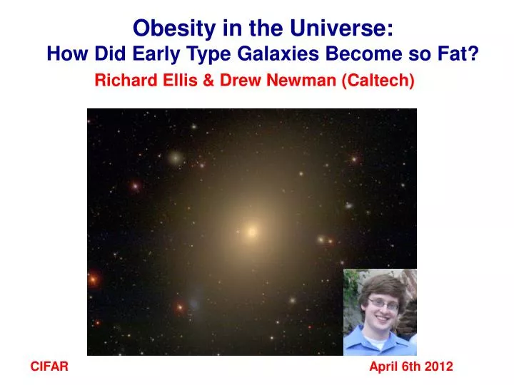
Obesity in the Universe: How Did Early Type Galaxies Become so Fat?. Richard Ellis & Drew Newman (Caltech). CIFAR April 6th 2012. Bimodal Galaxy Distribution. Star forming Blue Late type Young. Passive Red Early type Old. Bell et al. 2003.

E N D
Obesity in the Universe: How Did Early Type Galaxies Become so Fat? Richard Ellis & Drew Newman (Caltech) CIFAR April 6th 2012
Bimodal Galaxy Distribution Star forming Blue Late type Young Passive Red Early type Old Bell et al. 2003 • Hubble Sequence - morphology shows dynamically distinct populations Gas content/integrated colors - different ages and star formation histories
Color-magnitude Relation at z~2 Photometric and dynamical studies of early-type galaxies over 0<z<1 confirm that the most massive examples formed the bulk of their stars prior to z~2 And, sure enough, red and dead galaxies were eventually found at z~2 Logically these would seem to be the precursors of most of today’s massive early-types (although continued formation is also possible) Kriek et al 2009 Ap J 705, L71
Modest Increase in Mass Density of Red Galaxies Log Fractional Contribution to Total Stellar Mass 0.4<z<1.4 Spectroscopically-complete surveys of galaxies with IR-based stellar masses show only a modest increase (30%) in the abundance of M>1011M red galaxies over 0.4<z<1.4 (5 Gyr) at the expense of truncated SF in blue galaxies Rising Reds Declining Blues Bundy et al Ap J 651, 120 (2006)
The big surprise: z~2 early-types are SMALL! HST sizes of a representative sample of z~2-3 red galaxies with M >1011 M: re~0.9 kpc 2-5 times smaller than comparably massive z~0 ellipticals! Growth in size but not mass? half-light radius SDSS van Dokkum et al (2008) Earlier claims by: Daddi et al (2005), Trujillo et al (2006) 2 < z < 3
The `Red Nuggets’ Problem Initial skepticism at observational claims: result depends on combination of photometrically-determined masses and HST sizes of distant galaxies • Perhaps mass overestimated e.g. “bottom light” IMF, AGB stars • Perhaps size underestimated due to surface brightness effects • Dynamical data to confirm masses • Improved HST data over 0<z<2 • How much growth occurred in self-consistent samples? • Separating growth of long-lived populations vs new arrivals • What does it all mean?!
How Big Should a Massive Galaxy Be? Ask a Theorist Wuyts et al 2010 Ap J 722, 1666
Size Depends: I – On Gas Fraction of Initial Merger increasing dissipational gas fraction fgas local spheroids z~2 red galaxies re ~ exp( -fgas/0.3) fgas Equal mass merger SPH simulations using GADGET-2 with gas cooling, multi- phase ISM and SN/AGN feedback (Springel, Hernquist et al) Remnant is smaller for suitably-scaled z~3 disks with high gas fractions Wuyts et al 2010 Ap J 722, 1666
Size Depends: II – On Epoch of Merger Since gas fraction fgas declines with time, later merger products are larger NB: In principle this could account for expansion in size from z~2 to 0 but such a simple explanation is ruled out by low rate of major merging and absence of significant decline in abundance of fixed mass spheroids for z<1 Hopkins et al 2010 MN 401, 1099
Keck LRIS-R: IAB<23.5; 12-16 hr exposures, 1.1 < z < 1.60 Newman et al 2010 Ap J 707, L103
Size evolution at fixed dynamical mass Standard test conducted in literature: size ~ (1+z)-x Unlikely evolutionary path For M>1011 M x = 0.70 ± 0.11 (40% by z=1) • Only massive early-types are significantly growing in size • z > 2 objects appear ultra-compact implying very fast growth??
Size evolution at fixed velocity dispersion More physically meaningful Mergers should increase size but not velocity dispersion Exploits unique dynamical data Tests “progenitor bias” (cut in Mdyn restricts in σ, R so could give false evolutionary trend) For σ > 225 km s-1 x = 0.69 ± 0.21 Growth ×1.7-2.7 since z~2 Matched SDSS=LRIS Growth KeckSDSS Treu et al DEIMOS Cappellari stack van Dokkum z=2.2 Newman et al LRIS-R
Size Growth Rate in CANDELS data Size growth for 1011 M galaxy of × 3.5 ± 0.3 over 0.4 < z < 2.5 But scatter (1σ region) is significant (and valuable information) Growth rate consistent with that found in limited dynamical data and, again, particularly rapid in 2 Gyr period from 1.5<z<2.5 Newman et al (2012) Ap J 746, 162
How Did Early Galaxies Enlarge? • Improved observational data (dynamical masses, HST images) confirms size growth is real! • What, physically, could lead • to this growth in size? • Major mergers • Minor mergers • Mass loss/adiabatic expansion • (implausible as inactive systems)
Size Growth During Dissipationless Merging From virial theorem, total energy Consider merger such that and define Assuming conservation of energy (e.g. parabolic orbits, Binney & Tremaine 2008) Major merger : no change in v, M and R double, d log R / d log M = 1 Lots of minor mergers find d log R / d log M = 2 SPH simulations of minor mergers indicate d log R / d log M ~ 1.3 – 1.6 Naab et al 2009 Ap J 699, L108 (see also Khochfar & Silk 2006 Ap J 648, L21; Khochfar & Silk 2009 MNRAS 397, 506)
Measuring the Minor Merger Rate in CANDELS Data Satellite photo z precision WFC3/IR data is sufficiently deep (H<26.5) that we can secure photometric redshifts for secondaries 1/10th as massive for 404 quiescent primaries with log MP/M < 10.7 over 0.4 < z < 2 Search area 10 < R < 30 h-1 kpc δz < 0.1 (for z < 1) and δz < 0.2 (for 1 < z < 2) Mass ratio μ = MS/MP > 0.1 Caution: such photo-z associations could still lead to an over-estimate of pairs that will ultimately merge given environs in which red galaxies lie
Measuring the Minor Merger Rate in CANDELS Data Find fpair = 0.16 ± 0.03 over full z range μ*=0.3 μ*=0.5 μ*=0.2 Majority of secondaries are also red μ*=0.1 μ (mass ratio) distribution quite flat as expected from SAMs μ*=0.1 Newman et al (2012) Ap J 746, 162
Can Minor Merging Explain Size Growth: I? • Assuming: • Merger timescale • τe ~ 1-2 Gyr • (Patton+, Lotz+, Kitzbichler+) • 2. Bound fraction of projected pairs • Cmg (=f3D)~0.5 • 3. Size growth per mass increase • dlogR / dlogM ~1.6 • (Nipoti+) Size growth over 0.4<z<1 is broadly consistent with that expected from observer minor merger fraction IF merger timescale is fast Size growth over 1<z<2 is inconsistent with observed minor merger fraction for any reasonable choice of parameters
Accounting for New Arrivals Comoving no. density of log M>10.7 quiescents Simple model is naïve as it assumes all sources enlarge in lockstep from z~2 progenitors. In reality population comprises old galaxies which formed at z~2 and perhaps expand via mergers AND Newly arrived quiescent systems whose size reflects their epoch of formation Rapid size growth at high z may be associated with increase in no. density over 1.5<z<2.5
Evolution in Size Distribution Function Key to distinguishing growth of pre-existing sources and the arrival of new sources is the cumulative distribution of mass-normalized radius γ Cumulative Distribution Function (CDF) is fit by a skew-normal distribution at various redshifts In addition to matching the evolution in mean size growth and number density of quiescent galaxies, a satisfactory model must also account for the rate of depletion of the most compact systems from high redshift to low redshift.
A Two Phase Growth Model Consider CDF at z~2 and z~1: Mergers add mass and lead to enlargement. For “intra sample mergers”, the number also declines. Plausible model will shift some fraction P of the most compact z~2 sources to lie within the z~1 CDF with the remainder (1-P) as `new arrivals’ Defines Δlog γmin The test is thus whether the observed rate of minor mergers can deplete this fraction of the most compact sources in the observed CDFs
Can Minor Merging Explain Growth: II ? Conclusion unchanged: 0.4<z<1 size evolution is readily explained by observed rate of minor mergers, but rapid growth over 1<z<2.5 is harder to understand Newman et al (2012) Ap J 746, 162
Summary • Present-day massive early type galaxies formed most of their stars by z~2 • Evolving stellar mass functions place some limits on the continued appearance of massive early types: most are not genuine `new arrivals’ but represent some combination of dry mergers and truncated star formation in massive blue galaxies • The compact nature of early types at z~2.5 is confirmed by CANDELS data; we observe a × 3.5 growth in mean size over 0.4<z<2.5 for quiescent systems with masses > 1010.7 M. • Dynamical data has been key in verifying the relevant masses, at least to z~1.6; the `red nugget puzzle’ is unlikely to be due to observational errors/mis-interpretations • Minor mergers are so far the only plausible mechanism for the size growth. Modeling suggests the observed merger rate can explain the growth observed since z~1 but explaining the rapid growth observed over 1.5<z<2.5 remains a challenge
Cosmology with the Subaru Prime Focus Spectrograph http://sumire.ipmu.jp/en/2652
PFS Concept is Caltech/JPL WFMOS design Fiber connector mounted on top end structure Prime Focus Unit includes Wide Field Corrector (WFC) and Fiber Positioner. Spectrograph room located above Naysmith platform Design study based on Subaru-provided details, several visits to Subaru, interaction with HSC team Key requirements: survey speed and positioner reliability Fiber Cable routed around elevation axis and brings light to the Spectrographs
PFS Positioner Positioner Unit - Cobra A&G Fiber Guides Optical Bench with Positioner Units Cobra system tested at JPL in partnership with New Scale Technologies Designed to achieve 5μm accuracy in < 8 iterations (40 sec) 2400 positioners 8mm apart in hexagonal pattern to enable field tiling
Positioner Element – “Cobra” Top View Patrol Region • 7.7mm diameter, theta-phi system positioning within 9.5mm patrol area to 5μm precision. • Optical fibers mounted in “fiber arm” which attaches to upper postioner axis: • Fiber runs through the center of the positioner Fiber arm Second axis of rotation Phi stage First axis of rotation Fiber Tip Theta stage
Triple-arm Spectrograph (one of 4) Unique feature of Jim Gunn design is continuous coverage from 370nm to 1.3μm with matched spectral resolutions (R~2500-4000) for effective simultaneous exposures Detectors: Hamamatsu red-sensivity CCDs and expected Teledyne HgCdTe 4RG arrays
PFS Cosmology: Key Science Goals(Takada, Hirata, Kneib) • Measure the cosmological distances, DA(z) and H(z), to 3% accuracy in each of 6 redshift bins over 0.8<z<2.4 via the BAO experiment • Use the BAO distance constraints to reconstruct the dark energy densities in each redshift bin • Use the BAO distance constraints to constrain the curvature parameter ΩK to 0.3% accuracy • Measure the redshift-space distortion (RSD) effect to reconstruct the growth rate in each redshift bin to 6% accuracy
PFS Cosmology Survey • Assume 100 clear nights to meet the scientific goals → the area of PFS survey • The total volume: ~9 (Gpc/h)3 ~ 2 × BOSS survey • Assumed galaxy bias (poorly known): b=0.9+0.4z • PFS survey will have ngP(k)~a few@k=0.1Mpc/h in each of 6 redshift bins
Expected BAO constraints BOSS PFS-Red PFS-NIR • The PFS cosmology survey enables a 3% accuracy of measuring DA(z) and H(z) in each of 6 redshift bins, over 0.8<z<2.4 • This accuracy is comparable with BOSS, but extending to higher redshift range • Also very efficient given competitive situation • BOSS (2.5m): 5 yrs • PFS (8.2m): 100 nights
DE constraints • The BAO geometrical constraints achieved significantly constrain the DE parameters • For a (w0, wa)-DE model, H(z) and DA(z) are given as • PFS can significantly improve the DE constraints over BOSS • PFS can achieve a 0.3% accuracy of the curvature → a fundamental discovery • A wider redshift coverage as well as more independent z-bins are powerful aspects in improving the overall constraints (which the CMB alone cannot)
DE reconstruction • The wide-z coverage of PFS+BOSS enables a reconstruction of DE densities as a function of redshift → can constrain a broader range of DE models • PFS can significantly improve the accuracy of the reconstruction due to the increased z-bins • 7% accuracy of Ωde(z) in each of z-bins • PFS+SDSS+Planck allows a detection of dark energy up to z~2, for a Λ-type model
But is PFS competitive with BigBOSS? • Survey parameters taken from BigBOSS proposal • 500 vs. 100 nights • 14,000 vs. 1,420 deg2 • Naively, a factor (10)1/2 difference • BigBOSS better than PFS at z<1.2 (but note target selection a big issue for BigBOSS) • PFS comparable with BigBOSS for 1.2<z<1.6 but PFS can uniquely target1.6<z<2.4 • PFS more likely to complete its survey before Euclid BigBOSS (4m) vs. PFS (8.2m) BigBOSS
Redshift-Space Distortion (RSD) Peacock et al (2dF team, 01) • The redshift-space distortion can probe the growth rate • It gives a complementary probe of DE and can test gravity on cosmological scales • The PFS can reconstruct the growth rate in each of redshift bins, to a 7% accuracy