Download
1 / 29
290 likes | 403 Views
Hierarchical Model-based Autonomic Control of Software Systems. Marin Litoiu, IBM CAS Toronto Murray Woodside, Tao Zheng, Carleton University. Outline. Motivation Hierarchical Control Performance Models Conclusions. Client. Client. Data Server. Data Server. Web Server. Web Server.

E N D
Hierarchical Model-based Autonomic Control of Software Systems Marin Litoiu, IBM CAS Toronto Murray Woodside, Tao Zheng, Carleton University
Outline • Motivation • Hierarchical Control • Performance Models • Conclusions DEAS 05, St. Louis
Client Client Data Server Data Server Web Server Web Server App Server App Server Client Client A Typical Deployment: Data Centres SLAs component Application Data Centre DEAS 05, St. Louis
Response time time Self - optimization • Automated allocation of software and hardware resources to accomplish a performance goal by optimizing a cost function in the presence of • Workload variations • Perturbations • Change in the environment • Aims at • Reducing the cost of ownership • Improve the QoS (dependability) DEAS 05, St. Louis
Outline • Motivation • Hierarchical Control • Performance Models • Conclusions DEAS 05, St. Louis
Hierarchical Control(1) SLO SLO • Level 1: Component tuning • Level 2: Application tuning • Level 3: Provisioning DEAS 05, St. Louis
Hierarchical Control(2) DEAS 05, St. Louis
Hierarchical Control(3) • The Controller • Monitor the managed component performance metrics and the input workload and setpoints (SLOs) • Use the performance model to estimate future metrics and future adjustments of controlled parameters • If the future workloads cannot be accommodated by local adjustments, alert the upper level; otherwise perform the local adjustments. DEAS 05, St. Louis
Hierarchical Control(4): Advantages “When in doubt, mumble; when in trouble, delegate; when in charge, ponder.” • The targeted systems are hierarchical • Structure is hierarchical (containment) • Goals are hierarchical • Authority is hierarchical • Provides several homeostatic control levers: If the 1st one fails, engage the 2nd, if the 2nd one fails, engage the 3rd… • Solves time scale and scope issues • Reduces cognition, control and communication complexity DEAS 05, St. Louis
Agenda • Motivation • Hierarchical control • Performance Models • Conclusions DEAS 05, St. Louis
The Role of Performance Models • “All models are wrong, some models are useful.” • Prediction (forecast) role: tell what happens in the future • if the workload increases by 100 users, the response time will increase by 5s • Estimation role: what happens now • If I increase the number of threads, servers, alter the software architecture, what is the estimated change in performance • Problem determination role • Where is the bottleneck DEAS 05, St. Louis
Client Data Server Web Server App Server Client Queuing Network Models Di=service demand; X=throughput Ui=utilization of device i Qi=queue length at device i X=N/(R) Ui=X *Di DEAS 05, St. Louis
Client Client Data Server CPU, Disk Web Server CPU, Disk App Server CPU, Disk Client CPU, Disk Layered Queuing Models (LQM) • Layered Queuing Models (LQM) are analytic performance models that • Extend Queuing Network Models (QNMs) • Model queuing at software components: threading and data connection pools, locks and critical sections • Model multiple classes of requests • LQM Structure • Software resource interactions: synchronous, asynchronous, forward call • Demands at hardware resources for each class of request, one user per class in the system • Queuing centers: CPU, DISK, network, threading and data connections pools… Layer 1 Layer 0 DEAS 05, St. Louis
Linearized Dynamic Models • Linear regression models x(k)=Ax(k-1)+Bu(k) y(k)=Cx(k)+Du(k) x,u, y - vectors A,B,C,D- matrixes • Consider multiple input, output and state variables • Take into account the tendencies • Advantage • Take advantage of the controller design techniques from system control • Capture the transient behaviour Disadvantage • Assume the system is linear • The matrixes A,B,C,D are experimentally identified • Any change in the system will invalidate the model R(N)=C*N DEAS 05, St. Louis
Threshold and Policy Models • Decision is part of the Model • Monitor an output variable (utilization, queue length..) • Increase/decrease a state variable • “ If the number of users increases by 10, increase the number of threads by 5” • “ if the utilization is greater than 50%, then provision a new server” • More complex models • Monitor more output variables • Increase/decrease one output variable • Advantages • Very simple • Very fast • Disadvantages • Not globally optimal, sometimes not even locally optimal • Not able to handle changes in the system DEAS 05, St. Louis
Tradeoffs.……. • Layered Queuing Models • Model non-linearities across wide domains • Appropriate at application and system level • Work with mean values • Difficult to obtain service times per individual transactions( Kalman filters seem to help) • Dynamic Models • Model transitory behaviour • Appropriate at component level • For mean values, can be deduced from LQMs • In general, built experimentally (hard) • Enable System Control • Threshold and Policy Models • Can capture rules of thumb and domain experience • Can be deduced from the queuing or dynamic models • Appropriate at any level, as a default model • Simple and fast • Hard to maintain… DEAS 05, St. Louis
Conclusions • Hierarchical control • Solves the problem of timescale and scope • Provide flexibility of choice of control algorithms • Supports accelerated decision making by LQM at upper levels • Self Optimization=Component tuning + Application Tuning (Load balancing) + Provisioning • Models for Self-optimization • Threshold or Policy Based Models • Linearized Dynamic Models • Network or Layered Queuing Models • Further Work: • End to end evaluation • Optimization • Stability DEAS 05, St. Louis
Backup slides DEAS 05, St. Louis
Model Builder Prediction: = previous estimate of x ŷ = prediction of observation y based on and the model, Feedback: z = new observation vector = K ( z - ŷ ) * DEAS 05, St. Louis
Dynamic Models link AC to System Control Automatic Control 1952: Bellman’s optimal control (dynamic programming) 1878: Maxwell's “On Governors” 1931: Black&Nyquist’s electronic negative feedback amplifier 1789: Watt’s fly-ball governor 1960: Kalman fillter Experimental AC Classic AC Modern AC Autonomic Computing 2001:AC 1970’s: Time Sharing OS 1978: Cerf et al. TCP/IP DEAS 05, St. Louis
Solvers for LQMs • Algorithms • Layers of QNMs • The output of a lower lever is used as input for the upper level • Continue until a fix-point is reached • Public Solvers • Method of Layers (Rolia, Sevcik) • Based on Linearizer approximation algorithm • LQNS (Woodside ) • Based on approximate MVA • APERA (Litoiu) • Based on approximate MVA, two layers, on alphaworks Layer 2 Layer 1 Layer 0 (hardware) DEAS 05, St. Louis
LQMs- Predicting the application response time • Depending on the class mix, response time varies widely even when the number of users is constant ( 800) • Each class may reach its maximum response time for a different workload mix • Workload mixes produce changes in the bottlenecks DEAS 05, St. Louis
Monitored number of threads with HTTPConnection: Keep-Alive Estimated average number of threads Monitored number of threads with HTTPConnection:close LQMs- Predicting the Threading Level in WAS* • 100 clients ------------------------------- * From Litoiu M., "Migrating to Web services: a performance engineering approach," Journal of Software Maintenance and Evolution: Research and Practice, No 16, pp. 51-70, 2004. DEAS 05, St. Louis
Dynamic Models link AC to System Control Automatic Control 1952: Bellman’s optimal control (dynamic programming) 1878: Maxwell's “On Governors” 1931: Black&Nyquist’s electronic negative feedback amplifier 1789: Watt’s fly-ball governor 1960: Kalman fillter Experimental AC Classic AC Modern AC Autonomic Computing 2001:AC 1970’s: Time Sharing OS 1978: Cerf et al. TCP/IP DEAS 05, St. Louis
Component tuning • Example of control parameters • Threading level • Admission control • Scheduling • Session length • Live versus closed connections • Specialized controllers • Specialized decision making • How general can you be at the component level? • How can one systematically inject variability at this level? DEAS 05, St. Louis
Application tuning • Load balancing • horizontal scaling • vertical scaling • Inter-component optimization • DB2 connection pool in WAS • Component allocation • Scheduling • Controller and models • Become more complex • Become more general DEAS 05, St. Louis
Provisioning • Hardware and software provisioning • Add/remove hardware • Add/remove software components • Needs long term prediction DEAS 05, St. Louis
Building Accurate Models “If the map and the terrain don’t match, trust the terrain." Swiss Army Rule DEAS 05, St. Louis
THANKS! DEAS 05, St. Louis