Download
1 / 19
190 likes | 326 Views
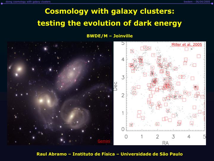
Cosmology with galaxy clusters: testing the evolution of dark energy. BWDE/M – Joinville. Miller et al. 2005. Gemini. Raul Abramo – Instituto de Física – Universidade de São Paulo. Summary.

E N D
Cosmology with galaxy clusters: testing the evolution of dark energy BWDE/M – Joinville Miller et al. 2005 Gemini Raul Abramo – Instituto de Física – Universidade de São Paulo
Summary • Galaxy clusters are the largest virialized structures in the Universe. They are rich is gas (both hot and ionized as well as cold gas) as well as cold dark matter. • The hot gas can be detected through the Sunyaev-Zeldovich effect, i.e., inverse compton scattering of the CMB photons off the hot intracluster electrons. This non-thermal effect leaves a characteristic imprint on the (originally) planckian spectrum. • Hot gas can also be detected, at high concentrations, through its X-ray emission (brehmsstrahlung). • The total (baryons + CDM) amount of matter in a cluster can be detected through weak (e.g. shear) and strong (e.g. Einstein ring) lensing. • Cold gas can also be detected through the hydrogen absorption spectra if a background quasar is available. • Clusters are great tools to study Cosmology! What about Dark Energy?
1. How clusters help pinpoint Dark Energy: that “little extra mile” Allen et al. 2004 WMAP 2003
Constraints from future SZe surveys Carlstrom, Holder & Reese 2002
Constraints from cosmic shear Jain & Taylor 2004 Effective depth to measure w of a shear survey, compared to other observations Ferguson & Bridle 2005
Kamionkowski & Loeb 1997, Cooray & Baumann 2002 2. Cluster Polarization and DE • The map of the CMB temperature fluctuations are essencially the portrait of a two-dimensional surface (the LSS) of radius R=hr . [h: conformal time; dh = dt/a(t) ] • In the presence of DE, the large-scale gravitational potential decays when DE starts to dominate. CMB photons propagating to us through space fall in and out of these time-changing potentials, gaining (or losing) energy. [Integrated Sachs-Wolfe effect – ISWe] F (z>>1) • It is hard to actually use the ISWe to extract information about the equation of state, since we cannot know in principle what in the CMB is due to the SW (intrinsic, at the LSS) effect and what is due to the ISWe. F (z<1) • We can use the Sunyaev-Zeldovich effect, which induces a polarization on the CMB photons that scatter off free electrons in galaxy clusters, to determine the ISWe. We can also use this polarization signal to make a tomography of the 3D spectrum of fluctuations!
CMB Bennett et al. ApJS 148:1 (2003)
What goes into the alm that we measure today: 1. Sachs-Wolfe effect:
2. ISWe: Crittenden & Turok 1997
Consider now a cluster at the direction Wc and at redshift zc. What kind of CMB would an observer in that cluster observe? • Spherical harmonic at cluster:
How can we in fact measure the alm‘s or the Cl‘s in clusters? • Sunyaev-Zeldovich effect Sunyaev & Zeldovich 80,81 Sazonov & Sunyaev 99 Hot ionized gas in clusters affects CMB photons through inverse Compton effect: The scattering also polarizes the CMB photons according to the quadrupole of the CMB temperature seen by the cluster. If we ignore the ISWe, the Q and U polarization modes for a cluster at position (q,j) are given by: • x=hn/kT , • f(x) is a spectral correction (of order 1), • t is the optical depth of the cluster, • lx and ly are linear combinations (eigenvalues) of the components of the quadrupole (a20, a21, a22) at the location of the cluster.
These clusters appear to us as “mini-quadrupoles” through the polarized CMB photons. This means that, if the CMB quadrupole isconstant, the degree and orientation of the SZe-induced polarization of clusters along a given line of sight does not vary with redshift (except for Cosmic Variance). However, in the presence of DE we know that the quadrupole evolved quite a lot, recently (z<~2) because of the ISWe. Therefore, with independent data (thermal SZe, X-ray) about the optical depth of a given cluster, the polarization of the CMB in the direction of clusters is a witness to the redshift-dependent quadrupole of the CMB.
Computing the Cl ’s for redshift bins and averaging over their positions will give: Effect is stronger for the quadrupole (l=2). If we measure the change of the quadrupole with time, we set limits over Fl (k,hc) and the growth function, g(z). This is a strong test of DE.
The time variation for the low multipoles (l<10) is very sensitive to the decay of the gravitational potentials: We can estimate how this test determines the parameters Wm and w through the function g’(z):
Efficacy of the observations Assuming a survey of clusters down to 1014 MO, with sensitivity for polarization of 0.1 mK, over 104 deg2 : Baumann & Cooray 2004
2. Polarization tomography Let’s return to the expression for the harmonic components, and let me assume for simplicity that the ISWe is small, so only the SWe remains: where Notice that the harmonic components are essentially functions of the position of the cluster, and are quite similar to a Fourier transform. Let’s invert this: Where
Using the completeness of Bessel’s functions and doing some algebra we get: Summing over m=-l,...,l we obtain: Where
For the quadrupole, the weight function which multiplies the spectrum is approximately peaked at cos g = ± 1 . Therefore, up to an approximation which can be easily improved, we can reconstruct the 3-dimensional spectrum of fluctuations by measuring the harmonic components in space (through cluster polarization). The final result: Therefore, if we can measure with some accuracy the quadrupole in galaxy clusters up to relatively high redshifts (z3), then we will be able to reconstruct the three-dimensional density field inside our LSS volume – and not only the two-dimensional spectrum on the LSS surface!