Download
1 / 7
70 likes | 196 Views
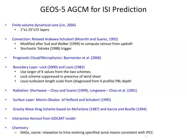
GEOS-5 AGCM for ISI Prediction. Finite volume dynamical core (Lin, 2004) 1 ° x1.25 ° x72 layers Convection: Relaxed Arakawa-Schubert ( Moorthi and Suarez, 1992) Modified after Sud and Walker (1999) to compute rainout from updraft Stochastic Tokioka (1988) trigger

E N D
GEOS-5 AGCM for ISI Prediction • Finite volume dynamical core (Lin, 2004) • 1°x1.25°x72 layers • Convection: Relaxed Arakawa-Schubert (Moorthi and Suarez, 1992) • Modified after Sud and Walker (1999) to compute rainout from updraft • Stochastic Tokioka (1988) trigger • Prognostic Cloud/Microphysics: Bacmeister et al. (2006) • Boundary Layer: Lock (2000) and Louis (1982) • Use larger of K values from the two schemes • Lock scheme suppressed in presence of wind shear • Louis turbulent length scale from (diagnosed from K profile) PBL depth • Radiation: Shortwave – Chou and Suarez (1999), Longwave – Chou et al. (2001) • Surface Layer: Monin-Obukov of Helfand and Schubert (1995) • Gravity Wave Drag Scheme based on McFarlane (1987) and Garcia and Boville (1994) • Interactive Aerosol from GOCART model • Chemistry • GHGs, ozone: relaxation to time evolving specified zonal means consistent with IPCC
The GEOS-5 OGCM for ISI Prediction • MOM4 • Version 4.1 patch 1 • ½°x½°x40 levels (1/4° equatorial refinement), tri-polar grid • B-grid, Z-coordinate (geopotential option) • KPP vertical mixing • Laplacian horizontal diffusion and friction • Diurnal skin layer (Price) • Sea ice: CICE (Los Alamos National Laboratory)
GEOS-5 AOGCM Coupling Configuration Atmospheric Model on AGCM Grid (GEOS-5) Momentum, Heat, Moisture fluxes, Gas Exchanges Surface Wind, Air Temperature, Specific Humidity, other atmos constituents All air-sea exchanges are implicit in time Air-sea Interface Component On Exchange grid Sea Ice Thermodynamics (CICE) Diurnal Layer (Price) Momentum, Heat , Fresh Water, and Salt Fluxes Gas Exchanges Mixed Layer Currents, Temperature, Salinity, etc Ocean Model on OGCM Grid Ocean Dynamics and Transport (MOM4) Sea Ice Dynamics (CICE) Ocean Radiation (NOMB) Ocean Biology (NOMB)
GEOS ODAS-2 • ODAS-2 can be run as an Ensemble Kalman Filter (EnKF) with state-dependent multivariate background error covariances or as an Ensemble OI (EnOI) with static multivariate background error covariances • EnKF: 20 member ensemble • EnOI: Static ensemble of 20 EOFs from time series of differences in 20-member ensemble AOGCM simulation • T and S profiles (Buoys, XBTs, CTDs, Argo) and Reynolds SST are assimilated daily. • XBT temperature profiles have been corrected according to Levitus et al. (2009). • For XBTs and Buoys, synthetic salinity profiles are generated from Levitus & Boyer S(T) • Climatological SSS is assimilated to compensate for errors in fresh water input from precipitation and river runoff. • Sea Level Anomalies are from AVISO. • Analysis is also constrained by Levitus & Boyer climatological temperature and salinity – correction made to first guess fields before assimilation of other real-time data – univariate. • Multivariate covariances correct T and S, not currents.
GEOS-5 Coupled analysis cycle for Initialization of ISI Predictions Relaxation to atmospheric states from MERRA (6-hourly) Precipitation corrected to GPCPv2.1 pentads (for LSM initialization) Initialized States for unconstrained coupled forecasts Precipitation corrected to GPCPv2.1 pentads (for LSM initialization) GEOS-5 AOGCM integration … AGCM … … … OGCM Ocean analysis EnKF & EnOI
Two-sided breeding in a coupled system – restarts from weakly coupled assimilation – positive and negative BVs – 1-month forecast restarts from perturbed coupled runs δ/2 rescaled bred vector δ +δ/2 unperturbed forecast ★ ★ ★ ★ -δ/2 1 month ★ • Bred vectors : 0.5* difference between the coupled forecast with positive perturbation and the coupled forecast with negative perturbation (accounts for model drift). • Coupled breeding cycle needs to choose physically meaningful breeding parameters in order to choose the type of instability • For seasonal prediction: BV_SST=0.1C in Niño3 region and rescaled every month Courtesy: Shu-Chih Yang
Seasonal Forecast strategy with GEOS-5 9-month duration Seasonal Forecasts 1 6 11 16 21 27 Jan Feb Mar Apr….. 1982 1983 ⡇ 1990 ⡇ 2011 Seasonal ensembles: 1st of month: Bred Vector perturbations (1-month rescaling) and/or coupled EnKF perturbations Later initialization to subsample subseasonal evolution in initial conditions Forecast anomalies calculated relative to ensemble climatological drift for each start date