Download
1 / 28
280 likes | 303 Views
Explore state-space modeling principles, exponential smoothing, prediction intervals, model selection, and outlier detection using random error terms. Understand the essential components and applications in financial modeling.

E N D
Chapter 5 State-Space Models for Time Series
Chapter 5: State-Space Models for Time Series 5.1 State-Space Models for Exponential Smoothing 5.2 The Random Error Term 5.3 Prediction Intervals from State-Space Models 5.4 Model Selection 5.5 Outliers 5.6 State-Space Modeling Principles
5.1 State-Space Models for Exponential Smoothing Models and Methods • AMethodprovides point forecasts, but does not provide any measures of uncertainty. • AModelis required to generate prediction intervals by specifying the dependence structure and an error process. A state space modelconsists of two parts: • An observation equation that relates the random variables (Yt) to the underlying state variable(s). • One or more state equations that describe how the state variable(s) evolve(s) over time. These equations involve the underlying random error process, which we denote by εt.
5.1 State-Space Models for Exponential Smoothing A State-Space Model for Simple Exponential Smoothing • Given an underlying level (state variable), Lt , we may formulate the observation equation as: • The level (state variable) is updated from one period to the next using the state equation: • The level represents the part that is known and the error the part that is unknown. Hence the model gives rise to the forecast function: Question: How does the process work? Construct a flow diagram showing how the parts are connected.
5.1 State-Space Models for Exponential Smoothing Example: The Random Walk • Consider this model for the special case . We arrive at the model: • That is, the latest value is the best forecast for the current period. This model for the stock market was first proposed by Louis Bachelier in 1900. It is now the foundation for the Efficient Markets Hypothesis (EMH) in financial modeling.
5.1 State-Space Models for Exponential Smoothing A Class of State-Space Models (Holt-Winters Additive Scheme) • Forecast function: • Observation equation: • State equations:
5.1 State-Space Models for Exponential Smoothing A Class of State-Space Models Mix and match components: • Trend (T): none (N), additive (A), Multiplicative (M), or damped (D) • Seasonal (S): none (N), additive (A) or multiplicative (M) • Error (E): additive (A) or multiplicative (M) Describe model byETS(., ., .) Table 5.1 Pegels’ Classification
5.3 Prediction Intervals from State-Space Models • The expected value of the next observation is given by the latest level and the one-step-ahead variance is constant, given the assumptions in Table 5.2: • The one-step-ahead prediction interval may be written as Forecast +/- ZRMSE: • Similarly, the h-step-ahead prediction interval is (see Appendix 5A for details):
5.3 Prediction Intervals from State-Space Models Prediction Intervals for the Local-Level Model: WFJ Sales Figure 5.1 Actual Values and Prediction Intervals for Observations 27–36 of WFJ Sales
5.3 Prediction Intervals from State-Space Models Prediction Intervals for the Local-Level Model: WFJ Sales Table 5.3 90 Percent Prediction Intervals for WFJ Sales (One to ten steps ahead from forecast origin week 26, fitted observations 1–26 and yielding = 0.728)
5.3 Prediction Intervals from State-Space Models Prediction Intervals for the Local-Level Model: Netflix Sales Table 5.4 95 Percent Prediction Intervals for Netflix Sales (1-8 steps ahead from forecast origin 2-13Q4)
5.3 Prediction Intervals from State-Space Models Prediction Intervals for the Local-Level Model: Netflix Sales Figure 5.2 95 Percent Prediction Intervals for Netflix Sales (1-8 steps ahead from forecast origin 2-13Q4)
5.4 Model Selection Two approaches: • Look for the model with the best performance over the hold-out sample [section 5.4.1] • Use a Penalty Function [section 5.4.2] based upon the estimation sample • error measures based upon the estimation sample suggest a “better fit” for more complicated models [e.g. loss of degrees of freedom in a regression model] • The idea underlying the use of a penalty function is that we compensate for this bias by adding a penalty term to the Mean Square error function that we seek to minimize • The resulting function is known as an Information Criterion • Select the model with the minimum value of the Information Criterion
5.4 Model Selection Netflix Sales (Table 5.5) Panel A: Parameter Estimates for Each Estimation Sample Use of a rolling origin with the hold-out sample Panel B: Forecast Errors
5.4 Model Selection Netflix Sales (Table 5.5 continued) Panel C: Summary Statistics Use of a rolling origin with the hold-out sample Discussion Question • In many forecasting applications, why is forecasting seasonality critically important?
5.4 Model Selection Information Criteria Select the model with the minimum value of the Information Criterion: IC = ln(MSE) + pQ(n) When the model involves a transformation, we transform back to the original units before calculating the IC. This procedure is heuristic in that it is not justified theoretically, but proves to be a useful comparative measure when different transformations (or none) are to be evaluated. Akaike’s information criterion (AIC; Akaike, 1971): Bayesian information criterion (BIC; Schwartz, 1978): Bias corrected AIC (AICc; Sugiura, 1978): Note that different programs formulate these criteria in somewhat different ways. The numbers change but the relative ordering of the models should not.
5.4 Model Selection Information Criteria: Netflix Sample Table 5.6 Values of the AIC and BIC Criteria for Different Models for the Netflix Data Discussion Question • How might you modify AIC and BIC if you wished to select the best model for forecasting h steps ahead?
5.4 Model Selection Automatic Model Selection Most leading software programs provide methods for automatic model selection, which is useful when large number of series must be forecast. Typically, they employ one or other of the two approaches just discussed. Discussion Question • If you were responsible for developing forecasting methods for a large number of data series (such as grocery store products), what combination of hold-out samples and information criteria would you employ?
5.5 Outliers An outlieris an extreme observation that, if not adjusted, may cause serious estimation and forecasting errors. Figure 5.3 Typical Patterns for Additive Outlier and Level Shift
5.5 Outliers • Plot the Z-scores for the original series and for the first differences; That is, and the equivalent in first differences. The original series is used to check for Additive Outlier (AO) and the differenced series for Level Shift (LS). • Find the first absolute Z-value that exceeds 3.0. If there are no such values, end the search. • If the observation with the extreme Z-value suggests a pattern such as either of those shown in Figure 5.3A or 5.3C, an AO is suggested. If either of Figures 5.3B and 5.3D is more appropriate, consider an LS. • Replace the outlier by a suitable reduced value; we suggest replacing the current Z-score by 1.5, with the same sign as the original. That is, for AO the new value is ; replace the positive sign with a negative sign when the Z-score is negative. For Level Shift (LS), apply the same adjustment to first differences. • Return to step 1 and continue until no outliers remain.
5.5 Outliers Dulles Example Table 5.7 Original and Adjusted Dulles Series for 1983–8 Table 5.8 Summary Results for Dulles Passenger Series, Without and With an Adjustment for the 1986 Outlier
5.6 State-Space Modeling Principles • Plot the series (or a sample of series). • Identify all the relevant features of the series. • Select the best performing model, using an information criterion and/or a hold-out sample. • Check the model assumptions. • Check for outliers and make adjustments where appropriate. • Examine the prediction intervals • and whether the hold-out sample falls within the interval.
Take-Aways • Use a forecasting model as the basis for making both point and interval forecasts • Examine the series to determine whether the model should include state variables to describe trend and/or seasonal factors. • Examine model performance by means of a hold-out sample whenever possible. • Check the validity of the model using diagnostic procedures.
Minicase 5.1 Analysis of UK Retail Sales The file UK_retail_sales_2.xlsx contains the quarterly index for the volume of total retail trade in the UK from 1996Q1 to 2014Q4. The index is not seasonally adjusted, and the index has 2010 as the base year with the index for that year set at 100. The file UK_retail_sales_annual.xlsxgives yearly figures for the same index, from 1955–2014 with an index value of 100 for 2010. • Determine the most appropriate models for forecasting both the quarterly and annual time series, and compare your forecasts from each approach for the complete years 2013 and 2014 (i.e., compare aggregate quarterly with annual). • Do the forecasts fall within appropriate prediction intervals? • Advanced: How would you generate prediction intervals for the forecasts you obtained by aggregation? Extend the data set to include the most recent data and rework the analysis for the last two years.
Minicase 5.2 Prediction Intervals for WFJ Sales We make use of the data file WFJ_sales.xlsx. Around week 12, the WFJ Sales manager changed the advertising strategy for the product, which resulted in an increase in sales. • To allow for this change, drop the first 12 observations and recompute the prediction intervals for weeks 27-36, using only observations 13-25 as the estimation sample. You will find that the RMSE is reduced and the width of the intervals increases more slowly, because αis smaller. • Repeat this analysis for other subsamples to see how the prediction intervals depend critically upon validating the assumptions listed in Table 5.2.
Appendix 5A: Derivation of Forecast Means and Variances • The general form of the error for the h-step-ahead forecast may be written as: • Since the errors are assumed to be independent and to have the same variance, it follows that the variance for the h-step-ahead forecast is: . • For the local-level model Aj= α, for all j = 1, 2, …So that the h-step-ahead variance in this case is: Question: What can be said about the variance as h increases?
Appendix 5B: State-Space Models with Multiplicative Seasonals (Holt-Winters Multiplicative Scheme) • Forecast function: • Observation equation: • State equations: