Download
1 / 12
120 likes | 265 Views
Ch 9: Maxwell’s Relations and Mixtures. I. General Thermodynamic Eqns. Given expt conditions, we want an eqn for a fundamental thermodynamic property as a function of its natural variables and then finding the associated extremum eqn.

E N D
I. General Thermodynamic Eqns • Given expt conditions, we want an eqn for a fundamental thermodynamic property as a function of its natural variables and then finding the associated extremum eqn. • Define degree of freedom (= X = extensive variable) and conjugate driving force (= P). • E.g. dU = Σ Pj dXj where Pj = (∂U/∂Xj)Xi≠j • Use the math tool, Legendre Transform, to do this.
Legendre Transforms (Ch 8) • Transform y = f(x) to a function expressed in terms of c(x) = dy/dx = slopes and b(x) = intercepts. • Start with y(x) = f(x) = c(x) x + b(x) and dy(x) = (dy/dx)dx = c(x)dx • Transform to b(x) = y(x) – c(x) x and db(x) = dy(x) – c(x) dx - x dc(x) = -x dc(x) • Ex. 9.1 and 9.2; Prob 8.1
II. Maxwell’s Relations • Handout • These relations or eqns allow us to “…predict nonmeasurable thermodynamic quantities from measurable ones” p 155 • More Applications – Chapter 9 Tools are presented in the next 3 slides as MR (Maxwell’s Relations) 1, 2, 3
MR 1: (∂U/∂V)T • How does U change with V at constant T?: Use dU = T dS - p dV (IIa) • Then (∂U/∂V)T = πT = T(∂S/∂V)T – p = T(∂p/∂T)V – p Note: LHS = nonmeas. But RHS = meas. • Try Ideal G. L., van der Waals G. L. • Ex 9.5
MR 2: (∂S/∂ℓ)T,p • Example 9.3
MR 3: Measurable α and к • α = (1/V) (∂V/∂T)p = thermal expansion coefficient; units = K-1; Fig 9.2 • к = - (1/V) (∂V/∂p)T = isothermal compressibility; units = atm-1 ; Fig 9.4 • Unusual behavior of water: Fig 9.5 (low α) and Fig 9.6 (low and negative к) due to H-bonds. Prob 9.2 • Ex 9.4 S = f(p) and Ex 9.5 U = f(V)
III. Mixtures • Now consider a system with more than one component. How do we determine how the amount of each component affects a particular total property at constant T and p? • Partial molar [Property] = (∂Prop/∂nj)T, p, ni • This partial describes how Prop changes with moles of the jth component, all other variables kept constant.
Partial Molar Volume • Partial molar volume = vj = (∂V/∂nj)T, p, ni This tells us how the total volume V changes as nj moles of component j are added. • Then V = Σ vjnj • dV = Σ(∂V/∂nj)T, p, ni dnj = Σ vjdnj
Calculating Total Volume • A mixture of one mol of water (v = 18.0 mL) and one mol of ethanol (v = 58.3 mL) are mixed. What are the partial volumes of water and alcohol? What is the total volume of this mixture?
Chemical Potential • Eqn 9.24 presents four expressions for chemical potential. Each one describes how the thermodynamic function varies with composition. • But the partial free function is the one at constant T and p. • Partial molar free energy = (∂G/∂Nj)T, p, Ni = μj = (∂H/∂Nj)T, p, Ni -T (∂S/∂Nj)T, p, Ni
More Applications – Ch 9 Tools • Gibbs Duhem Eqn tells us that partial molar quantities (from homogenous thermo fnts) are related and how they are linked. • Σ njdvj = 0 at const p, T Eqn 9.33 • Also Σ Njdμj = 0 at const p, T Eqn 9.37