Download
1 / 66
820 likes | 1.26k Views
Lecture 6 Oceanographic Applications: Ocean Color. IoE 184 - The Basics of Satellite Oceanography. 6. Oceanographic Applications: Ocean color observations. This lecture includes the following topics:. 1. Basic principles of satellite measurements of ocean color;.

E N D
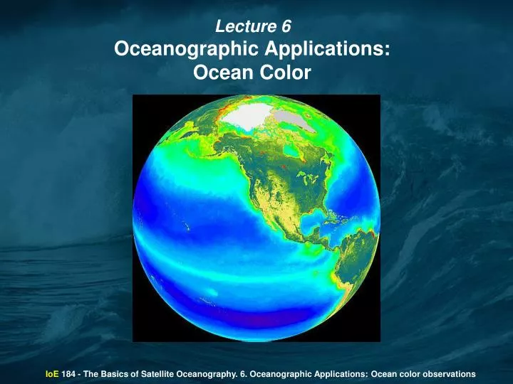
Lecture 6 Oceanographic Applications: Ocean Color IoE 184 - The Basics of Satellite Oceanography. 6. Oceanographic Applications: Ocean color observations
This lecture includes the following topics: 1. Basic principles of satellite measurements of ocean color; 2. Coastal Zone Color Scanner (CZCS); 3. Sea-viewing Wide Field-of-view Sensor (SeaWiFS); 4. MODerate resolution Imaging Spectroradiometer (MODIS); 5. Patterns of phytoplankton distribution in World Ocean obtained from ocean color. IoE 184 - The Basics of Satellite Oceanography. 6. Oceanographic Applications: Ocean color observations
1. Basic principles of satellite measurements of ocean color The measurements of ocean color are based on electromagnetic energy of 400-700 nm wavelength. This energy is emitted by the sun, transmitted through the atmosphere and reflected by the earth surface. IoE 184 - The Basics of Satellite Oceanography. 6. Oceanographic Applications: Ocean color observations
1. Basic principles of satellite measurements of ocean color The sunlight is not merely reflected from the sea surface. The color of water surface results from sunlight that has entered the ocean, been selectively absorbed, scattered and reflected by phytoplankton and other suspended material in the upper layers, and then backscattered through the surface. IoE 184 - The Basics of Satellite Oceanography. 6. Oceanographic Applications: Ocean color observations
1. Basic principles of satellite measurements of ocean color Unlike observations in the infrared, where the radiation is emitted from the top 10-100 µm of the sea surface, ocean color radiances in the blue-green can be upwellied from the depth as great as 50 m. The transparency of clean open ocean water is very high; the upper layer of tens of meters depth contributes to ocean color, this contribution decreasing with depth. IoE 184 - The Basics of Satellite Oceanography. 6. Oceanographic Applications: Ocean color observations
1. Basic principles of satellite measurements of ocean color In turbid coastal waters the depth of the upper layer decreases to few meters and less. IoE 184 - The Basics of Satellite Oceanography. 6. Oceanographic Applications: Ocean color observations
1. Basic principles of satellite measurements of ocean color The color of ocean surface depends on the color of the sunlight transmitted through the atmosphere. IoE 184 - The Basics of Satellite Oceanography. 6. Oceanographic Applications: Ocean color observations
1. Basic principles of satellite measurements of ocean color The color of water surface is regulated by the color of pure ocean water and the concentrations of different types of particles suspended in the upper water layer. At this aerial photograph you see that in the coastal zone high concentrations of phytoplankton and suspended matter change water color. IoE 184 - The Basics of Satellite Oceanography. 6. Oceanographic Applications: Ocean color observations
1. Basic principles of satellite measurements of ocean color Water color depends on chlorophyll concentration, which in turn depends on phytoplankton biomass. IoE 184 - The Basics of Satellite Oceanography. 6. Oceanographic Applications: Ocean color observations
1. Basic principles of satellite measurements of ocean color The change of water color is also evident at satellite true-color images. IoE 184 - The Basics of Satellite Oceanography. 6. Oceanographic Applications: Ocean color observations
1. Basic principles of satellite measurements of ocean color Clean ocean water absorbs red light, i.e., sun radiation of long wavelength and transmits and scatters the light of short wavelength. That is why ocean surface looks blue. Phytoplankton cells contain chlorophyll that absorbs other wavelengths and contributes green color to ocean water. In coastal area suspended inorganic matter backscatters sunlight, contributing green, yellow and brown to water color. IoE 184 - The Basics of Satellite Oceanography. 6. Oceanographic Applications: Ocean color observations
1. Basic principles of satellite measurements of ocean color Thus, color (including water color) can be measured on the basis of the spectrum of visible light emitted from the study object. Clean ocean water (A) has maximum in short (blue) wavelength and almost zero in yellow and red. Higher is phytoplankton (i.e., chlorophyll and other plant pigments) concentration, more is contribution of green color (B). In coastal zones with high concentration of dead organic and inorganic matter light spectrum has maximum in red (C). IoE 184 - The Basics of Satellite Oceanography. 6. Oceanographic Applications: Ocean color observations
1. Basic principles of satellite measurements of ocean color • The sources of color change in seawater include: • Phytoplankton and its pigments • Dissolved organic material • Colored Dissolved Organic Material (CDOM, or yellow matter, or gelbstoff) is derived from decaying vegetable matter (land) and phytoplankton degraded by grazing of photolysis. • Suspended particulate matter • The organic particulates (detritus) consist of phytoplankton and zooplankton cell fragments and zooplankton fecal pellets. • The inorganic particulates consist of sand and dust created by erosion of land-based rocks and soils. These enter the ocean through: • River runoff. • Deposition of wind-blown dust. • Wave or current suspension of bottom sediments. IoE 184 - The Basics of Satellite Oceanography. 6. Oceanographic Applications: Ocean color observations
1. Basic principles of satellite measurements of ocean color Both CDOM and particulates absorb sunlight strongly in the blue waveband, yielding a brownish yellow color to the water. IoE 184 - The Basics of Satellite Oceanography. 6. Oceanographic Applications: Ocean color observations
1. Basic principles of satellite measurements of ocean color Given the density of dissolved and suspended material, Morel and Prieur (1977) divide the ocean into case 1 and case 2 waters. In case 1 waters, phytoplankton pigments and their co-varying detrital pigments dominate the seawater optical properties. In case 2 waters, other substances that do not co-vary with Chl-a (such as suspended sediments, organic particles, and CDOM) are dominant. Even though case 2 waters occupy a smaller area of the world ocean than case 1 waters, because they occur in coastal regions with large river runoff and high densities of human activities such as fisheries, recreation and shipping, they are equally important. IoE 184 - The Basics of Satellite Oceanography. 6. Oceanographic Applications: Ocean color observations
1. Basic principles of satellite measurements of ocean color For most regions of the world, the color of the ocean is determined primarily by the abundance of phytoplankton and associated photosynthetic pigments. IoE 184 - The Basics of Satellite Oceanography. 6. Oceanographic Applications: Ocean color observations
1. Basic principles of satellite measurements of ocean color The subsurface reflectance R(λ) depends on backscattering b(λ) and absorption a(λ) of different compounds. R(λ) = G • b(λ) / a(λ) Where G is a constant that depends on the incident light field. Different wavelengths are important to observe CDOM, chlorophyll and fluorescence. Chlorophyll absorption peak is at 443 nm; CDOM-dominated wavelength is at 410 nm; Measurements must also be made in the 500-550 nm range where the chlorophyll absorption is zero and the absorption of other plant pigments (I.e., carotenoids) dominate. Fluorescence requires observations in the vicinity of 683-nm peak. IoE 184 - The Basics of Satellite Oceanography. 6. Oceanographic Applications: Ocean color observations
1. Basic principles of satellite measurements of ocean color Sunlight backscattered by the atmosphere contributes 80-90% of the radiance measured by a satellite sensor at visible wavelengths. Such scattering arises from dust particles and other aerosols, and from molecular (Rayleigh) scattering. However, the atmospheric contribution can be calculated and removed if additional measurements are made in the red and near-infrared spectral regions (e.g., 670 and 750 nm). Since blue ocean water reflects very little radiation at these longer wavelengths, the radiance measured is due almost entirely to scattering by the atmosphere. Long-wavelength measurements, combined with the predictions of models of atmospheric properties, can therefore be used to remove the contribution to the signal from aerosol and molecular scattering. IoE 184 - The Basics of Satellite Oceanography. 6. Oceanographic Applications: Ocean color observations
1. Basic principles of satellite measurements of ocean color • First step of atmospheric correction is cloud detection, based on a threshold in the near-infrared waveband. • The algorithms of atmospheric correction estimate the contribution to the signal: • Ozone • The distribution of ozone is determined by Total Ozone Mapping Spectrometer (TOMS) instrument on the Earthprobe satellite and similat instrument on EOS-AURA satellite launched in 2004 • Sun glint • Is a function of sun angle and wind speed • Foam • Also depends on wind speed and to less extent of sun angle • Rayleigh path radiances (I.e., scattering by air molecules) • Aerosol path radiances (most complex part of the algorithm) • Based on “black pixel” assumption • Diffuse transmittance • Estimates signal contamination from land and ice IoE 184 - The Basics of Satellite Oceanography. 6. Oceanographic Applications: Ocean color observations
CZCS = Coastal Zone Color Scanner (1978 - 1986) SeaWiFS = Sea-viewing Wide Field-of-view Sensor (since 1997) MODIS = Moderate Resolution Imaging Spectroradiometer Terra Satellite launched December 18th, 1999 Aqua satellite launched May 4th, 2002. Three water color sensors are of great significance for oceanography: IoE 184 - The Basics of Satellite Oceanography. 6. Oceanographic Applications: Ocean color observations
2. Coastal Zone Color Scanner (CZCS) The Coastal Zone Color Scanner (CZCS), was a multi-spectral line scanner developed by NASA to measure ocean color as a means of determining chlorophyll concentrations and the distributions of particulate matter and dissolved substances. IoE 184 - The Basics of Satellite Oceanography. 6. Oceanographic Applications: Ocean color observations
2. Coastal Zone Color Scanner (CZCS) CZCS was launched aboard Nimbus-7 satellite platform in October 1978. Due to the power demands of the various on-board experiments the CZCS operated on an intermittent schedule. The infra-red/temperature sensor (channel 6 - 10.5-12.5 microns) failed within the first year. Nominal orbit parameters for the Nimbus-7 spacecraft are: Launch date 10/24/1978 Orbit Sun-synchronous, near polar Nominal Altitude (km) 955 Inclination (deg) 104.9 Nodal Period (min.) 104 Equator Crossing Time 1200 noon (ascending) Nodal Increment (deg) 26.1 IoE 184 - The Basics of Satellite Oceanography. 6. Oceanographic Applications: Ocean color observations
2. Coastal Zone Color Scanner (CZCS) The following lists the sensor's channels and the primary purpose of each: Reflected solar energy was measured in 5 channels: 1 433-453 nm (blue) chlorophyll absorption 2 510-530 nm (green) chlorophyll concentration 3 540-560 nm (yellow) Gelbstoffe concentration 4 660-680 nm (red) aerosol absorption 5 700-800 nm (far red) land and cloud detection Infrared radiation was measured in one channel: 6 10.5-12.5 microns (infra-red) surface temperature IoE 184 - The Basics of Satellite Oceanography. 6. Oceanographic Applications: Ocean color observations
2. Coastal Zone Color Scanner (CZCS) The CZCS had a scan width of 1556 km centered on nadir and the ground resolution was 0.825 km at nadir. The scenes (images) obtained by CZCS are partial orbital swaths. In one two-minute data segment, the CZCS covers approximately 1.3 million square kilometers of the ocean surface. CZCS collected about 60,000 images. IoE 184 - The Basics of Satellite Oceanography. 6. Oceanographic Applications: Ocean color observations
2. Coastal Zone Color Scanner (CZCS) Each scan of the CZCS viewed the Earth for approximately 27.5 microseconds. During this period, each channel of the analog data output was digitized to obtain a total of about 2000 samples. Successive scans occur at the rate of 8 per second. The archive of CZCS data products began with November 2, 1978 and continued until June 22, l986. However, there are several periods of intermittent coverage. When operating full time, approximately 400 images were collected each month. IoE 184 - The Basics of Satellite Oceanography. 6. Oceanographic Applications: Ocean color observations
2. Coastal Zone Color Scanner (CZCS) Level 1 data were processed to Level 2 – surface plant pigment concentrations. These Level 2 data were compiled onto daily, weekly and monthly mosaics (Level 3 data). Each Level 3 file is a fixed, linear latitude-longitude (equal angle) grid of dimension 1024 (latitude) x 2048 (longitude) with ~18.5 km resolution at the equator. Daily and weekly composites contain too few information to obtain a realistic global pattern of plant pigment distribution. IoE 184 - The Basics of Satellite Oceanography. 6. Oceanographic Applications: Ocean color observations
2. Coastal Zone Color Scanner (CZCS) Monthly Level 3 composites provide realistic patterns of phytoplankton concentration during 7.5 years (from November 1978 to June 1986). November 1978 IoE 184 - The Basics of Satellite Oceanography. 6. Oceanographic Applications: Ocean color observations
2. Coastal Zone Color Scanner (CZCS) Monthly Level 3 composites provide realistic patterns of phytoplankton concentration during 7.5 years (from November 1978 to June 1986). December 1978 IoE 184 - The Basics of Satellite Oceanography. 6. Oceanographic Applications: Ocean color observations
2. Coastal Zone Color Scanner (CZCS) Monthly Level 3 composites provide realistic patterns of phytoplankton concentration during 7.5 years (from November 1978 to June 1986). January 1979 IoE 184 - The Basics of Satellite Oceanography. 6. Oceanographic Applications: Ocean color observations
2. Coastal Zone Color Scanner (CZCS) Monthly Level 3 composites provide realistic patterns of phytoplankton concentration during 7.5 years (from November 1978 to June 1986). February 1979 IoE 184 - The Basics of Satellite Oceanography. 6. Oceanographic Applications: Ocean color observations
2. Coastal Zone Color Scanner (CZCS) Monthly Level 3 composites provide realistic patterns of phytoplankton concentration during 7.5 years (from November 1978 to June 1986). March 1979 IoE 184 - The Basics of Satellite Oceanography. 6. Oceanographic Applications: Ocean color observations
2. Coastal Zone Color Scanner (CZCS) Monthly Level 3 composites provide realistic patterns of phytoplankton concentration during 7.5 years (from November 1978 to June 1986). April 1979 IoE 184 - The Basics of Satellite Oceanography. 6. Oceanographic Applications: Ocean color observations
2. Coastal Zone Color Scanner (CZCS) Monthly Level 3 composites provide realistic patterns of phytoplankton concentration during 7.5 years (from November 1978 to June 1986). May 1979 IoE 184 - The Basics of Satellite Oceanography. 6. Oceanographic Applications: Ocean color observations
2. Coastal Zone Color Scanner (CZCS) Monthly Level 3 composites provide realistic patterns of phytoplankton concentration during 7.5 years (from November 1978 to June 1986). June 1979 IoE 184 - The Basics of Satellite Oceanography. 6. Oceanographic Applications: Ocean color observations
2. Coastal Zone Color Scanner (CZCS) Monthly Level 3 composites provide realistic patterns of phytoplankton concentration during 7.5 years (from November 1978 to June 1986). July 1979 IoE 184 - The Basics of Satellite Oceanography. 6. Oceanographic Applications: Ocean color observations
2. Coastal Zone Color Scanner (CZCS) Monthly Level 3 composites provide realistic patterns of phytoplankton concentration during 7.5 years (from November 1978 to June 1986). August 1979 IoE 184 - The Basics of Satellite Oceanography. 6. Oceanographic Applications: Ocean color observations
2. Coastal Zone Color Scanner (CZCS) Monthly Level 3 composites provide realistic patterns of phytoplankton concentration during 7.5 years (from November 1978 to June 1986). September 1979 IoE 184 - The Basics of Satellite Oceanography. 6. Oceanographic Applications: Ocean color observations
2. Coastal Zone Color Scanner (CZCS) Monthly Level 3 composites provide realistic patterns of phytoplankton concentration during 7.5 years (from November 1978 to June 1986). October 1979 IoE 184 - The Basics of Satellite Oceanography. 6. Oceanographic Applications: Ocean color observations
2. Coastal Zone Color Scanner (CZCS) Monthly Level 3 composites provide realistic patterns of phytoplankton concentration during 7.5 years (from November 1978 to June 1986). November 1979 IoE 184 - The Basics of Satellite Oceanography. 6. Oceanographic Applications: Ocean color observations
2. Coastal Zone Color Scanner (CZCS) Monthly Level 3 composites provide realistic patterns of phytoplankton concentration during 7.5 years (from November 1978 to June 1986). December 1979 IoE 184 - The Basics of Satellite Oceanography. 6. Oceanographic Applications: Ocean color observations
2. Coastal Zone Color Scanner (CZCS) This image shows total surface plant pigment concentration in the World Ocean averaged over the entire period of observations (November 1978 – June 1986). IoE 184 - The Basics of Satellite Oceanography. 6. Oceanographic Applications: Ocean color observations
2. Coastal Zone Color Scanner (CZCS) Access to CZCS data: CZCS data can be obtained from the website ftp://disc1.gsfc.nasa.gov/data/czcs/ It contains: Level 1A GAC data; Level 2 browse data (chlorophyll concentration); GAC data Level 3 Monthly data Level 1 data can be ordered from the website http://daac.gsfc.nasa.gov/data/datapool/CZCS/index.html IoE 184 - The Basics of Satellite Oceanography. 6. Oceanographic Applications: Ocean color observations
3. Sea-viewing Wide Field-of-view Sensor (SeaWiFS) The SeaWiFS program was started in 1980s, immediately after the end of the CZCS mission. The launch of the satellite was first planned on 1993, but the spacecraft was launched in 1997. The SeaWiFS radiometer and the OrbView-2 spacecraft were developed by ORBIMAGE Corporation in cooperation with NASA. IoE 184 - The Basics of Satellite Oceanography. 6. Oceanographic Applications: Ocean color observations
3. Sea-viewing Wide Field-of-view Sensor (SeaWiFS) OrbView-2 satellite was launched to low Earth orbit on board an extended Pegasus launch vehicle on August 1, 1997. IoE 184 - The Basics of Satellite Oceanography. 6. Oceanographic Applications: Ocean color observations
3. Sea-viewing Wide Field-of-view Sensor (SeaWiFS) Orbit Type Sun Synchronous Altitude 705 km Equator Crossing Noon +20 min descending Orbital Period 99 minutes Swath Width 2,801 km LAC/HRPT (58.3 degrees) 1,502 km GAC (45 degrees) Spatial Resolution 1.1 km LAC, 4.5 km GAC Mission Characteristics IoE 184 - The Basics of Satellite Oceanography. 6. Oceanographic Applications: Ocean color observations
3. Sea-viewing Wide Field-of-view Sensor (SeaWiFS) The swaths overlap in high latitudes and are separated in low latitudes. Thus, each location of the ocean is observed every other day. IoE 184 - The Basics of Satellite Oceanography. 6. Oceanographic Applications: Ocean color observations
3. Sea-viewing Wide Field-of-view Sensor (SeaWiFS) The OrbView-2 spacecraft navigation is a self-contained system, with complete information about the attitude of the spacecraft and its orbital position integrated into the downlinked data stream. Orbit determination is provided by on-board Global Positioning System (GPS) receivers. The GPS receivers yield 100 m position accuracy (after ground postprocessing). IoE 184 - The Basics of Satellite Oceanography. 6. Oceanographic Applications: Ocean color observations
3. Sea-viewing Wide Field-of-view Sensor (SeaWiFS) Instrument Bands Band Wavelength 1 402-422 nm 2 433-453 nm 3 480-500 nm 4 500-520 nm 5 545-565 nm 6 660-680 nm 7 745-785 nm 8 845-885 nm IoE 184 - The Basics of Satellite Oceanography. 6. Oceanographic Applications: Ocean color observations
3. Sea-viewing Wide Field-of-view Sensor (SeaWiFS) >130 (at April 2004) receiving stations receive Local Area Coverage (LAC) data from SeaWiFS and provide high-resolution (1 km) images to NASA Goddard Space Flight Center (GSFC) in Maryland. Global Area Coverage (GAC) data transmitted directly to GSFC have lower (4 km) resolution. IoE 184 - The Basics of Satellite Oceanography. 6. Oceanographic Applications: Ocean color observations
3. Sea-viewing Wide Field-of-view Sensor (SeaWiFS) There is an embargo period of 2 weeks from collection for general distribution of data to research users to protect ORBIMAGE's commercial interest. Access to the data is permitted for research purposes by authorized users. IoE 184 - The Basics of Satellite Oceanography. 6. Oceanographic Applications: Ocean color observations