Download
1 / 20
200 likes | 335 Views
Mixture Kalman Filters by Rong Chen & Jun Liu. Presented by Yusong Miao Dec. 10, 2003. Structure. Introduce the originals of the problem Mixture Kalman Filters (MKF) model setup and method Two related extended models w/ examples Applications to show the advantages of MKF Conclusions.

E N D
Mixture Kalman Filtersby Rong Chen & Jun Liu Presented by Yusong Miao Dec. 10, 2003
Structure • Introduce the originals of the problem • Mixture Kalman Filters (MKF) model setup and method • Two related extended models w/ examples • Applications to show the advantages of MKF • Conclusions
Original of the problem • Interest in on-line estimation and prediction of the dynamic changing system. (Hidden pattern along observations) • Kalman filter (1960) technique can OK Gaussian linear system. • How about non-linear & non-Gaussian system? • ------Sequential Monte Carlo approach including: Bootstrip filter / practical filter; Sequential imputation; • From on now, call it as “Monte Carlo filters” • ------Mixed kalman filter, the role of this paper. • Will see the comparisons.
Original of the problem • Before we start MKF, recall the task:
MKF model setup • Conditional dynamic linear model (CDLM): • Given trajectory of an indicator variable, the system is Gaussian & linear-- can derive a MC filter focusing on attention on the space of indicator variables, named Mixed Kalman Filter.
MKF model setup • Example 1: A special CDLM (Linear system with non-Gaussian errors) as the follow: • In the CDLM system MKF is more sophisticated, outperform other methods (i.e.. bootstrap filter). • Use a mixture of Gaussian distribution to estimate the target posterior distribution.
MKF model setup • The method of MKF • Use a weighted sample of the indicators: • To represent the distribution p(Λt|yt) a random mixture of Gaussian distribution: • Can approximate the target distribution p(xt|yt).
MKF model setup • Algorithm (updating weights)---If you are interested in:
Extended MKF with examples • Beside the situation of CDLM, there is a extended one called partial conditional dynamic linear models (PCDLM). • PCDLM are interested in non-linear component of state variables. • No absolute distinction between CDLM and PCDLM.
Extended MKF with examples • Example: Fading channel modeling system (mobile communication channel can be modeled as Rayleigh flat fading channels)
Extended MKF with examples • Example: Blind deconvolution digital communication system • Where St is a discrete process taking vales on a known set S. It is to be estimated from the observed signals {y1,…,yt}, without knowing the channel coefficients θi. • There two examples can be solved by extended MKF called EMKF.
Extended MKF with examples • Why EMKF? It can deal with as many linear and Gaussian components from systems as possible. • P(xt1,xt2|yt)=P(xt1|xt2,y)*P(xt2|yt), Monte Carlo approximation of P(xt2|yt) and an Gaussian conditional distribution p(xt1|xt2,y). • Need to generate discrete samples in the joint space of the indicators and the non-linear state components.
Extended MKF with examples • Algorithm (updating weights)
Application of MKF-Target tracking • Situation setup: • The tracking errors (differences between the estimated and true target location) are generated and compared with other methods.
Application of MKF-Target tracking • The result proves the advantage of MKF:
Application of MKF-2 D target’s position • A 2-D target’s position is sampled every T=10s. We know the movement and velocities on both x and y directions. Use MKF to simulate the results and compare them with the actual data. • Model setup:
Application of MKF-2 D target’s position • The result proves the advantage of MKF: • Better than the tradition way done by Bar-Shalom & Fortmann
Other applications of MKF • There are still several other applications with brief introduction can be found on the paper. • Random (non-Gaussian) accelerated target (no clutter). • Digital signal extraction in fading channels. • They are both improved under MKF approach comparing with traditional Monte Carlo approach.
Conclusions • MKF can perform real time estimation and prediction in CDLM situation, which outperform Sequential Monte Carlo approaches. • Similar to EMKF in PCDLM situation. • MKF can combine with other Monte Carlo techniques (Markov chain Monte Carlo updates, delayed estimation, fixed lag filter, etc.) to improve effectiveness. • Sequential Monte Carlo method can be a platform for designing efficient non-linear filtering algorithms.
Questions & Answers Thank you & Happy holiday!