Download
1 / 45
740 likes | 2.55k Views
Statistics for Business and Economics 6 th Edition Chapter 21 Statistical Decision Theory Chapter Goals After completing this chapter, you should be able to: Describe basic features of decision making Construct a payoff table and an opportunity-loss table

E N D
Statistics for Business and Economics6th Edition Chapter 21 Statistical Decision Theory Statistics for Business and Economics, 6e © 2007 Pearson Education, Inc.
Chapter Goals After completing this chapter, you should be able to: • Describe basic features of decision making • Construct a payoff table and an opportunity-loss table • Define and apply the expected monetary value criterion for decision making • Compute the value of sample information • Describe utility and attitudes toward risk Statistics for Business and Economics, 6e © 2007 Pearson Education, Inc.
Steps in Decision Making • List Alternative Courses of Action • Choices or actions • List States of Nature • Possible events or outcomes • Determine ‘Payoffs’ • Associate a Payoff with Each Event/Outcome combination • Adopt Decision Criteria • Evaluate Criteria for Selecting the Best Course of Action Statistics for Business and Economics, 6e © 2007 Pearson Education, Inc.
List Possible Actions or Events Two Methods of Listing PayoffTable Decision Tree Statistics for Business and Economics, 6e © 2007 Pearson Education, Inc.
Payoff Table • Form of a payoff table • Mij is the payoff that corresponds to action ai and state of nature sj Statistics for Business and Economics, 6e © 2007 Pearson Education, Inc.
Payoff Table Example A payoff table shows actions (alternatives), states of nature, and payoffs Statistics for Business and Economics, 6e © 2007 Pearson Education, Inc.
Decision Tree Example Strong Economy 200 Large factory Stable Economy 50 Weak Economy -120 Strong Economy 90 Average factory Stable Economy 120 Weak Economy -30 Strong Economy 40 Small factory Stable Economy 30 Weak Economy 20 Payoffs Statistics for Business and Economics, 6e © 2007 Pearson Education, Inc.
Decision Making Overview Decision Criteria * Nonprobabilistic Decision Criteria: Decision rules that can be applied if the probabilities of uncertain events are not known No probabilities known Probabilities are known • maximin criterion • minimax regret criterion Statistics for Business and Economics, 6e © 2007 Pearson Education, Inc.
The Maximin Criterion • Consider K actions a1, a2, . . ., aK and H possible states of nature s1, s2, . . ., sH • Let Mij denote the payoff corresponding to the ith action and jth state of nature • For each action, find the smallest possible payoff and denote the minimum M1* where • More generally, the smallest possible payoff for action ai is given by • Maximin criterion: select the action ai for which the corresponding Mi* is largest (that is, the action with thegreatest minimum payoff) Statistics for Business and Economics, 6e © 2007 Pearson Education, Inc.
Maximin Example • The maximin criterion • For each option, find the minimum payoff 1. Minimum Profit -120 -30 20 Statistics for Business and Economics, 6e © 2007 Pearson Education, Inc.
Maximin Solution (continued) • The maximin criterion • For each option, find the minimum payoff • Choose the option with the greatest minimum payoff 2. Greatest minimum is to choose Small factory 1. Minimum Profit -120 -30 20 Statistics for Business and Economics, 6e © 2007 Pearson Education, Inc.
Regret or Opportunity Loss • Suppose that a payoff table is arranged as a rectangular array, with rows corresponding to actions and columns to states of nature • If each payoff in the table is subtracted from the largest payoff in its column . . . • . . . the resulting array is called a regret table, or opportunity loss table Statistics for Business and Economics, 6e © 2007 Pearson Education, Inc.
Minimax Regret Criterion • Consider the regret table • For each row (action), find the maximum regret • Minimax regret criterion: Choose the action corresponding to the minimum of the maximum regrets (i.e., the action that produces the smallest possible opportunity loss) Statistics for Business and Economics, 6e © 2007 Pearson Education, Inc.
Opportunity Loss Example Opportunity loss (regret) is the difference between an actual payoff for a decision and the optimal payoff for that state of nature Payoff Table The choice “Average factory” has payoff 90 for “Strong Economy”. Given “Strong Economy”, the choice of “Large factory” would have given a payoff of 200, or 110 higher. Opportunity loss = 110 for this cell. Statistics for Business and Economics, 6e © 2007 Pearson Education, Inc.
Opportunity Loss (continued) Payoff Table Opportunity Loss Table Statistics for Business and Economics, 6e © 2007 Pearson Education, Inc.
Minimax Regret Example • The minimax regret criterion: • For each alternative, find the maximum opportunity loss (or “regret”) Opportunity Loss Table 1. Maximum Op. Loss 140 110 160 Statistics for Business and Economics, 6e © 2007 Pearson Education, Inc.
Minimax Regret Example (continued) • The minimax regret criterion: • For each alternative, find the maximum opportunity loss (or “regret”) • Choose the option with the smallest maximum loss Opportunity Loss Table 1. Maximum Op. Loss 2. Smallest maximum loss is to choose Average factory 140 110 160 Statistics for Business and Economics, 6e © 2007 Pearson Education, Inc.
Decision Making Overview Decision Criteria No probabilities known Probabilistic Decision Criteria: Consider the probabilities of uncertain events and select an alternative to maximize the expected payoff of minimize the expected loss * Probabilities are known • maximize expected monetary value Statistics for Business and Economics, 6e © 2007 Pearson Education, Inc.
Payoff Table • Form of a payoff table with probabilities • Each state of nature sj has an associated probability Pi Statistics for Business and Economics, 6e © 2007 Pearson Education, Inc.
Expected Monetary Value (EMV) Criterion • Consider possible actions a1, a2, . . ., aK and H states of nature • Let Mij denote the payoff corresponding to the ith action and jth state and Pj the probability of occurrence of the jth state of nature with • The expected monetary value of action ai is • The Expected Monetary Value Criterion: adopt the action with the largest expected monetary value Statistics for Business and Economics, 6e © 2007 Pearson Education, Inc.
Expected MonetaryValue Example • The expected monetary value is the weighted average payoff, given specified probabilities for each state of nature Suppose these probabilities have been assessed for these states of nature Statistics for Business and Economics, 6e © 2007 Pearson Education, Inc.
Expected Monetary Value Solution (continued) Goal: Maximize expected monetary value Example: EMV (Average factory) = 90(.3) + 120(.5) + (-30)(.2) = 81 Payoff Table: Maximize expected value by choosing Average factory Expected Values (EMV) 61 81 31 Statistics for Business and Economics, 6e © 2007 Pearson Education, Inc.
Decision Tree Analysis • A Decision tree shows a decision problem, beginning with the initial decision and ending will all possible outcomes and payoffs Use a square to denote decision nodes Use a circle to denote uncertain events Statistics for Business and Economics, 6e © 2007 Pearson Education, Inc.
Add Probabilities and Payoffs (continued) Strong Economy (.3) 200 Large factory Stable Economy (.5) 50 Weak Economy (.2) -120 (.3) Strong Economy 90 Average factory (.5) Stable Economy 120 (.2) Weak Economy -30 Decision (.3) Strong Economy 40 Small factory (.5) Stable Economy 30 (.2) Weak Economy 20 States of nature Probabilities Payoffs Statistics for Business and Economics, 6e © 2007 Pearson Education, Inc.
Fold Back the Tree Strong Economy (.3) EMV=200(.3)+50(.5)+(-120)(.2)=61 200 Large factory Stable Economy (.5) 50 Weak Economy (.2) -120 (.3) Strong Economy EMV=90(.3)+120(.5)+(-30)(.2)=81 90 Average factory (.5) Stable Economy 120 (.2) Weak Economy -30 (.3) Strong Economy EMV=40(.3)+30(.5)+20(.2)=31 40 Small factory (.5) Stable Economy 30 (.2) Weak Economy 20 Statistics for Business and Economics, 6e © 2007 Pearson Education, Inc.
Make the Decision Strong Economy (.3) EV=61 200 Large factory Stable Economy (.5) 50 Weak Economy (.2) -120 (.3) Strong Economy EV=81 90 Maximum EMV=81 Average factory (.5) Stable Economy 120 (.2) Weak Economy -30 (.3) Strong Economy EV=31 40 Small factory (.5) Stable Economy 30 (.2) Weak Economy 20 Statistics for Business and Economics, 6e © 2007 Pearson Education, Inc.
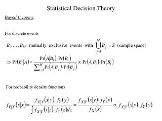
Bayes’ Theorem • Let s1, s2, . . ., sH be H mutually exclusive and collectively exhaustive events, corresponding to the H states of nature of a decision problem • Let A be some other event. Denote the conditional probability that si will occur, given that A occurs, by P(si|A) , and the probability of A , given si , by P(A|si) • Bayes’ Theorem states that the conditional probability of si, given A, can be expressed as • In the terminology of this section, P(si) is the prior probability of si and is modified to the posterior probability, P(si|A), given the sample information that event A has occurred Statistics for Business and Economics, 6e © 2007 Pearson Education, Inc.
Expected Value of Perfect Information, EVPI Perfect information corresponds to knowledge of which state of nature will arise • To determine the expected value of perfect information: • Determine which action will be chosen if only the prior probabilities P(s1), P(s2), . . ., P(sH) are used • For each possible state of nature, si, find the difference, Wi, between the payoff for the best choice of action, if it were known that state would arise, and the payoff for the action chosen if only prior probabilities are used • This is the value of perfect information, when it is known that si will occur Statistics for Business and Economics, 6e © 2007 Pearson Education, Inc.
Expected Value of Perfect Information, EVPI (continued) • The expected value of perfect information (EVPI) is • Another way to view the expected value of perfect information Expected Value of Perfect Information EVPI = Expected monetary value under certainty – expected monetary value of the best alternative Statistics for Business and Economics, 6e © 2007 Pearson Education, Inc.
Expected Value Under Certainty • Expected value under certainty = expected value of the best decision, given perfect information Value of best decision for each event: 200 120 20 Example: Best decision given “Strong Economy” is “Large factory” Statistics for Business and Economics, 6e © 2007 Pearson Education, Inc.
Expected Value Under Certainty (continued) • Now weight these outcomes with their probabilities to find the expected value: 200 120 20 200(.3)+120(.5)+20(.2) = 124 Expected value under certainty Statistics for Business and Economics, 6e © 2007 Pearson Education, Inc.
Expected Value of Perfect Information Expected Value of Perfect Information (EVPI) EVPI = Expected profit under certainty – Expected monetary value of the best decision Recall: Expected profit under certainty = 124 EMV is maximized by choosing “Average factory”, where EMV = 81 so: EVPI = 124 – 81 = 43 (EVPI is the maximum you would be willing to spend to obtain perfect information) Statistics for Business and Economics, 6e © 2007 Pearson Education, Inc.
Bayes’ Theorem Example Consider the choice of Stock A vs. Stock B Expected Return: 18.012.2 Stock A has a higher EMV Statistics for Business and Economics, 6e © 2007 Pearson Education, Inc.
Permits revising old probabilities based on new information Bayes’ Theorem Example (continued) Prior Probability New Information Revised Probability Statistics for Business and Economics, 6e © 2007 Pearson Education, Inc.
Bayes’ Theorem Example (continued) • Additional Information: Economic forecast is strong economy • When the economy was strong, the forecaster was correct 90% of the time. • When the economy was weak, the forecaster was correct 70% of the time. F1 = strong forecast F2 = weak forecast E1 = strong economy = 0.70 E2 = weak economy = 0.30 P(F1 | E1) = 0.90 P(F1 | E2) = 0.30 Prior probabilities from stock choice example Statistics for Business and Economics, 6e © 2007 Pearson Education, Inc.
Bayes’ Theorem Example (continued) • Revised Probabilities (Bayes’ Theorem) Statistics for Business and Economics, 6e © 2007 Pearson Education, Inc.
EMV with Revised Probabilities Σ = 25.0 Σ = 11.25 Revised probabilities EMV Stock B = 11.25 EMV Stock A = 25.0 Maximum EMV Statistics for Business and Economics, 6e © 2007 Pearson Education, Inc.
Expected Value of Sample Information, EVSI • Suppose there are K possible actions and H states of nature, s1, s2, . . ., sH • The decision-maker may obtain sample information. Let there be M possible sample results, A1, A2, . . . , AM • The expected value of sample information is obtained as follows: • Determine which action will be chosen if only the prior probabilities were used • Determine the probabilities of obtaining each sample result: Statistics for Business and Economics, 6e © 2007 Pearson Education, Inc.
Expected Value of Sample Information, EVSI (continued) • For each possible sample result, Ai, find the difference, Vi, between the expected monetary value for the optimal action and that for the action chosen if only the prior probabilities are used. • This is the value of the sample information, given that Ai was observed Statistics for Business and Economics, 6e © 2007 Pearson Education, Inc.
Utility • Utility is the pleasure or satisfaction obtained from an action • The utility of an outcome may not be the same for each individual • Utility units are arbitrary Statistics for Business and Economics, 6e © 2007 Pearson Education, Inc.
Utility (continued) • Example: each incremental $1 of profit does not have the same value to every individual: • Arisk averseperson, once reaching a goal, assigns less utility to each incremental $1 • A risk seeker assigns more utility to each incremental $1 • A risk neutral person assigns the same utility to each extra $1 Statistics for Business and Economics, 6e © 2007 Pearson Education, Inc.
Three Types of Utility Curves Utility Utility Utility $ $ $ Risk Seeker Risk-Neutral Risk Aversion Statistics for Business and Economics, 6e © 2007 Pearson Education, Inc.
Maximizing Expected Utility • Making decisions in terms of utility, not $ • Translate $ outcomes into utility outcomes • Calculate expected utilities for each action • Choose the action to maximize expected utility Statistics for Business and Economics, 6e © 2007 Pearson Education, Inc.
The Expected Utility Criterion • Consider K possible actions, a1, a2, . . ., aK and H states of nature. • Let Uij denote the utility corresponding to the ith action and jth state and Pj the probability of occurrence of the jth state of nature • Then the expected utility, EU(ai), of the action ai is • The expected utility criterion: choose the action to maximize expected utility • If the decision-maker is indifferent to risk, the expected utility criterion and expected monetary value criterion are equivalent Statistics for Business and Economics, 6e © 2007 Pearson Education, Inc.
Chapter Summary • Described the payoff table and decision trees • Defined opportunity loss (regret) • Provided criteria for decision making • If no probabilities are known: maximin, minimax regret • When probabilities are known: expected monetary value • Introduced expected profit under certainty and the value of perfect information • Discussed decision making with sample information and Bayes’ theorem • Addressed the concept of utility Statistics for Business and Economics, 6e © 2007 Pearson Education, Inc.