Download
1 / 21
211 likes | 400 Views
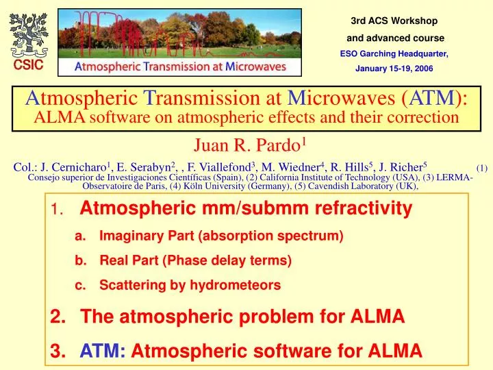
3rd ACS Workshop and advanced course ESO Garching Headquarter, January 15-19, 2006. A tmospheric T ransmission at M icrowaves ( ATM ): ALMA software on atmospheric effects and their correction. Juan R. Pardo 1

E N D
3rd ACS Workshop and advanced course ESO Garching Headquarter, January 15-19, 2006 Atmospheric Transmission at Microwaves (ATM): ALMA software on atmospheric effects and their correction Juan R. Pardo1 Col.: J. Cernicharo1, E. Serabyn2, , F. Viallefond3, M. Wiedner4, R. Hills5, J. Richer5(1) Consejo superior de Investigaciones Científicas (Spain), (2) California Institute of Technology (USA), (3) LERMA-Observatoire de Paris, (4) Köln University (Germany), (5) Cavendish Laboratory (UK), • Atmospheric mm/submm refractivity • Imaginary Part (absorption spectrum) • Real Part (Phase delay terms) • Scattering by hydrometeors • The atmospheric problem for ALMA • ATM: Atmospheric software for ALMA
1. Atmospheric mm/submm Refractivity 1.0 + Gas-phase contribution + Hydrometeros contribution Impact approximation collision << 1 / Van-Vleck-Weisskopf line profile 1c. Scattering. Polarization must be included 1a. Imaginary Part (absorption) 1a. Imaginary Part (absorption) 1b. Real Part (phase delay) ( ) I Q I= « Intensity vector » K: 2x2 matriz de extinción : vector de emisión K=2S+ S: 2x2 scattering matrix Chajnantor zenith transmission for 0.5 mm H2O / Water lines / Oxygen lines / ozone lines / H2O-foreign / N2-N2 + N2-O2 + O2-O2
1a. Atmospheric absorption • "Line" spectrum: rotational transitions of H2O, O2, O3, N2O, CO, and other trace gases. • "Hydrometeor" contribution: absorption & scattering by liquid, ice and other particles. • Collision-induced absorption by N2-N2, O2-O2 and N2-O2, H2O-N2, H2O-O2 mechanisms
1a. Atmospheric absorption: Direct measurements with FTS experiments at Mauna Kea, Chajnantor & Sout Pole • Accurately measure the shape of the terrestrial longwave spectrum. • Solve the « excess of continuum » problem. • Input to build an state-of-the-art absorption models: ARTS(Bremen University)AM(CfA, Harvard)ATM(CalTech, CSIC) Characteristics of CSO-FTS • Mounted on Cassegrain focus of telescope for dedicated obs. runs. • Detector: 3He cooled Bolometer • Moving arm: 50 cm ~ 200 MHz resolution • Filters: 7 different (165 to 1600 GHz) Schematics of FTS experiment
CSO-FTS: Some of the best data sets, subsequently used to study the collision-induced non-resonant absorption a ALMA overlap Zenith Transmission Frecuency (GHz)
Serabyn, Weisstein, Lis & Pardo, Appl. Optics, 37:2185, 1998 Matsushita, Matsuo, Pardo, & Radford, PASJ, 51:603, 1999. Pardo, Serabyn & Cernicharo, JQSRT, 68:419, 2001 Pardo, Cernicharo & Serabyn, IEEE TAP, 49:1683, 2001 Pardo, Wiedner, Serabyn, Wilson, Cunningham, Hills & Cernicharo, Ap. J. Suppl., 153:363, 2004 Pardo, Serabyn, Wiedner & Cernicharo, JQSRT, 96:537, 2005 The collision-induced non-resonant absorption a Absorption lines taken out in the analysis. Remaining absorption due to collision-induced non-resonant mechanisms Very important result for submm astronomy
Resulting model Example 1: Opacity terms in wet atmospheric conditions at Mauna Kea
Example 2: Atmospheric transmission at high frequencies in dry Mauna Kea conditions 1.0 0.8 0.6 Transmission 0.4 0.2 0.0 Frequency (GHz) Model (0.5 mm H2O)CSO data 3/98CSO data 7/99 Atacama data 6/98
1. Atmospheric mm/submm Refractivity 1.0 + Gas-phase contribution + Hydrometeros contribution Impact approximation collision << 1 / Van-Vleck-Weisskopf line profile 1c. Scattering. Polarization must be included 1a. Imaginary Part (absorption) 1b. Real Part (phase delay) 1b. Real Part (phase delay) ( ) I Q I= « Intensity vector » K: 2x2 matriz de extinción : vector de emisión K=2S+ S: 2x2 scattering matrix
1. Atmospheric mm/submm Refractivity 1.0 + Gas-phase contribution + Hydrometeros contribution Impact approximation collision << 1 / Van-Vleck-Weisskopf line profile 1c. Scattering. Polarization must be included 1c. Scattering. Polarization must be included 1a. Imaginary Part (absorption) 1b. Real Part (phase delay) ( ) I Q I= « Intensity vector » K: 2x2 matriz de extinción : vector de emisión K=2S+ S: 2x2 scattering matrix High cirrus (ice particles)
2. The atmospheric problem for ALMA atm a (baseline, wind, atmospheric status) ~ 20 m
Atmospheric water vapor fluctuations gas,i(x,y,z,t) P(x,y,z,t) T(x,y,z,t) Refractive index field n(x,y,z,t) : Line of sight coordinate t=t0; nd Flat ground for interferometry Antennae positions: (xi,yi) (Rxy)i Wavefront delay (x,y) (Rxy) < (rxy) (Rxy-rxy)> Radiative transfer along coordinate at t=t0 Delay autocorrelation functionA(Rxy) Atmospheric brightness temperatureTB(x,y) TB(Rxy) Power spectrum of delayP(qxy) P(qxy) 2D FT Frozen screen; y=0 x=vt A(t) ATB(t) Temporal autocorrelation functions TB autocorrelation functionATB(Rxy) 2D FT < TB(rxy) TB(Rxy-rxy)> Power spectrum of TBPTB(qxy) 1D FT P() PTB() All functions are dependent
Example of atmospheric water vapor field: Kolmogorov Screen With an interferomerter and a reference point source P(qxy)atastro PTB,()PH2O() P() With one antenna we can measure TB(t), from which we obtain: <TB(t') TB(t-t')> PTB,() Chose very sensitive to H2O so that we track PH2O() y (m) With two antennas: P() atastro
6km 70m 0 outer -5/3 2D -8/3 3D Kol Temporal Power Spectra: Px()The slope informs on the scale of phenomena 5km 500m 50m d for v=5 m/s PTB,() measured on Nov/25/2001 at Mauna Kea 1 = 183.317.8 GHz 2 = 183.313.0 GHz 3 = 183.311.3 GHz Outer sc. -5/3 2D -8/3 3D P()measured on Nov/25/2001 at Mauna Kea at astro = 230.5 GHz Target source: Uranus Base line: 48 m Instr. Time 1000s 100s 10s PTB,()PH2O() P() OK / 70 m - 6 km : 2D Kolmogorov screen
Phase correction can be performed using water vapor radiometry at frequencies sensitive to H2O 10.41 μm/μm 8.47 μm pathlength / μm PWV 6.65 μm/μm 612 μm 462 μm 353 μm Assuming 0.4 K noise in 1 s in all three channels of the Water Vapor Radiometer Uncertainty in determining the PWV: 2.3 μm The goal of 15 μm pathlength correction accuracy for ALMA should be reachable with this technique in time scales of the order of 1 s. CURRENT PROTOTYPES ALREADY MEET THESE REQUIREMENTS Taking an average Precipitable Water Vapor amount of 0.5 mm, we have: 23 mk/μm60 mk/μm 173 mk/μm
Phase fluctuations: Correction using 183 GHz water vapor radiometers Observing Frequency: 230.5 GHz, PWV to phase conversion factor: 1.944 deg/m a Time since the beginning of the observation (min) on Nov. 25, 2001
3. ATM: Atmospheric software for ALMA • Starting point: Fortran code developed during 20 years. • Contract with ESO to develop ATM for alma. • Fortran library created to encapsulate "fundamental" physics of the problem (C++). • C++ interface developed specifically for ALMA needs. • Updated via CVS. • Doxygen documented. • Test examples provided using real FTS and WVR data. • Work done withing the TelCal working group.
Old ATM fortran code Ground Temperature Tropospheric Lapse Rate Ground Pressure Rel. humidity (ground) Water vapor scale height Primary pressure step Pressure step factor Altitude of site Top of atmospheric profile ATM_telluric 1st guess of water vapor column Layer thickness (NPP) Number of atmospheric layers, NPP Layer pressure (NPP) Layer temperature (NPP) Layer water vapor (NPP) Layer_O3 (NPP) Layer CO (NPP) Layer N2O (NPP) User Other sources to obtain atmospheric parameters ATM_st76 ATM_rwat DATA_xx_lines DATA_xx_index xx all species ABSORPTION COEFS. kh2o_lines (NPP) kh2o_cont (NPP) ko2_lines (NPP) kdry_cont (NPP) kminor_gas (NPP) PHASE FACTORS total_dispersive_phase (NPP) total_nondisp_phase (NPP) INI_singlefreq ABS_h2oABS_o2 ABS_co ABS_o3_161618 ABS_h2o_v2ABS_o2_vib ABS_n2o ABS_o3_161816 ABS_hdoABS_16o17o ABS_o3 ABS_o3_nu1 ABS_hh17oABS_16o18o ABS_o3_161617 ABS_o3_nu2 ABS_hh18oABS_cont ABS_o3_161716 ABS_o3_nu3 kabs (NPP) Frequency Air mass Bgr. Temp. Applications: INV_telluric for WVR and FTS data (available in current release) RT_telluric Atmospheric radiance INTERFACE LEVEL I/O Parameters DEEP LEVEL(LIBRARY)
ALMA-ATM C++ structure: Collaboration diagram between the most important classes Design workshop: Tuesday afternoon Class AtmProfile: Profiles of physical conditions & chemical abundances Class AbsorptionPhaseProfile: Profiles of refractive index for an array of frequencies Class WaterVaporRadiometer: WVR system in place for phase correction Class SkyStatus: Relevant atmospheric information for antenna operations