Download
1 / 1
10 likes | 154 Views
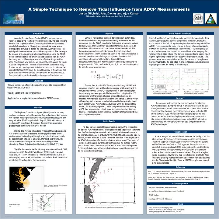
A Simple T echnique to Remove T idal I nfluence from ADCP Measurements Justin Gilchrist, Alex Davies and Ajoy Kumar. Millersville University, Department of Earth Sciences. Introduction. Methods. Initial Results Continued.

E N D
A Simple Technique to Remove Tidal Influence from ADCP Measurements Justin Gilchrist, Alex Davies and Ajoy Kumar.Millersville University, Department of Earth Sciences. Introduction Methods Initial Results Continued Similar to various other studies in de-tiding ocean current data, harmonic analysis was employed to both identify and remove the tidal component from the ROMS model data. In the case of harmonic analysis to identify tides, there were thirty-seven tidal harmonics that need to be considered. All harmonics and observations beyond these known tidal harmonics represent residual data or error. The thirty-seven tidal harmonics are well known and studied. Each of the tidal harmonics has a constant speed, or rates of change in the phase of the individual constituent, which are readily available through NOAA via tidesandcurrents.noaa.gov. Harmonic analysis begins by calculating the thirty-seven sets of tidal coefficients, Ak and Bk, for each of the data points for both the u and v components. Acoustic Doppler Current Profiler (ADCP) measured current velocities close to the coast are strongly influenced by the local tides and there lacks a simplistic method of removing this influence from vessel mounted observations. In this study, we demonstrate a new simple technique that allows us to de-tide the observed ADCP velocities. The technique is based on simple vector differencing method. The first step in the process is to produce tidal velocities of the region using the ROMS model. In the next step, we remove the tidal velocities from the ADCP data using vector differencing at a number of points along the ships track. An extensive error analysis will be carried out to assess the validity of our de-tiding methods. Two sets of points will be used in this study. The first set will contain points that lie inside the model domain and the second set of points that lie on the model boundary. In this way, we can determine the effect of the model boundaries on the above technique. Results will determine the feasibility and accuracy of the technique. Figure 4 and figure 5 compare the u and v components respectively. They also include the resulting de-tided components. In figure 4, the ROMS model seems to do a fair job representing the observed u-component of the ADCP. The v-components, found in figure 5, display a larger dissimilarity between the observed and modeled v-components. This discrepancy is a topic of further research and needs to be considered when analyzing the validity of the de-tided values. The de-tided components are, as one would expect, significantly smaller then the observed and modeled values. This provides some reassurance to that fact that the currents in the region are heavily influenced by the local tides. A proper statistical analysis is needed to properly evaluate the validity of this technique. Objectives The raw data from the ADCP was processed using VMDAS and converted into short term and long term averages, which span 5 and 15 minutes respectively. WinADCP was then used to convert those short term and long term averages into Matlab variables. Using the U and V components with the vessels influence removed the locations are matched with the model output for the same time period. A simple vector differencing method is used to estimate the de-tided current velocities at each location where ADCP data was available within the domain of the model. For this study, eighteen U and V components from the ancillary ADCP data were matched in both space and time with data points from ROMS . The resultant current velocities represent shelf currents with the tidal components removed. • Provide a simple yet effective technique to remove tidal component from vessel mounted ADCP data • Test the validity of the de-tiding technique • Apply method at varying depths as well as other BIOME cruises Figure 4: Plot of observed ADCP u component, ROMS u component and the de-tided u component. Figure 5: Plot of observed ADCP v component, ROMS v component and the de-tided v component. Summary In summary, we found that the best approach to de-tiding the ADCP data collected during the BIOME lV cruise would be with the use of a regional ocean model. Given the cruise track, it was found that the Chesapeake Bay Regional Ocean Model System would be the best fit for this particular study. Using harmonic analysis to identify the tidal currents we were able to use simple vector subtraction to remove the tidal component from the velocities collected by the ADCP. We look to continue to use this method to remove the tidal component from the ADCP data at depth. Materials The Regional Ocean Model System (ROMS) used in our study has been configured for the Chesapeake Bay and adjacent shelf regions with a terrain-following or orthogonal curvilinear coordinate system. This study will utilize ROMS output data for July 4-5, 2006 with a temporal resolution of 1 hour. Figure 1 visualizes this coordinate system in a gridded model domain with land areas masked BIOME (Bio-Physical Interactions in Coastal Margin Ecosystems) IV is one of a collection of seasonal oceanographic cruises, which monitor various meteorological, biological, and physical interactions in the coastal region offshore of Delaware, Maryland, and Virginia. The cruises observe and interpret the seasonal variability of these interactions. Figure 2 displays the ship track of the BIOME lV cruise. The ADCP data collected for this study was collected from BIOME cruises using a RD (Now RDI) “Workhorse” 600 KHz with a nominal range of 60 m. The 1st bin resided 2.11m beneath the surface. For all intensive purposes this will be considered the surface. Each successive been below the surface bin is 1 meter in width. Initial Results To date we have applied these concepts to get our first glimpse that the de-tided ADCP observations. We expected to see a significant shift in the direction from the original observations to the de-tided observations due to the strong tidal influence in and around the mouth of the Chesapeake bay. In addition, we also expected to see a substantial reduction in the magnitude of the ADCP observations after the tidal influence was removed. The results of Figure 3 (below) support our original hypotheses that the de-tided vectors (black) indeed show a directional shift as well as a reduction in magnitude. Further analysis is required to properly identify and inspect the vectors that did not support our hypothesis. Future Research • An error analysis will be carried out to estimate the validity of our de-tiding method. In addition, further comparisons will be made between The above steps will be again used at different depths to get a current profile of the inner shelf region. With a gridded field of the inner and outer shelf currents, ancillary BIOME cruise data can be used to identify coastal processes such as upwelling and relate them to satellite and biological data collected over the area of interest. The physical regime can be characterized by the CTD data collected during BIOME IV. Wind stress and upwelling indexes could also be estimated from data obtained from the Chesapeake Bay Light Tower and NDBC buoy located nearest to the cruise transect. References Wilks, D. S., Statistical Methods in the Atmospheric Sciences, 2nd Edition, International Geophysics Series, Vol. 91, ElsevierInc., Boston, 2006, Chaps. 8, 9. Press, W. H., Teukolsky, S. A., Vetterling, W. T., and Flannery, B. P., Numerical Recipes in C++, The Art of Scientific Computing, 2nd Edition, Cambridge University Press, New York, 2002, Chap. 2. Acknowledgements Figure 1: Display of the domain of the Chesapeake Bay ROMS used for this study. Millersville University Earth Sciences Department John and Tiffany Moisan - NASA Wallops Island Flight Facility M_MAP Tool Box Bruce Lipphardt, University of Delaware Figure 2: BOIME IV ship track Grants Figure 3: Vector plot of original ADCP observations (Black) and the de-tided observations (Red). Note that since this is a time series the data was collected over the course of two days. • AGU Student Travel Grant, Spring 2010 • Millersville University Student Research Grant, Spring 2009 • Neimeyer-Hodgson Student Research Grant, Fall 2008