Completely Randomized Design Experiments Steven Schuelka Director, MSQA Program

1. Completely Randomized Design Experiments Steven Schuelka Director, MSQA Program Calumet College of St. Joseph

2. Designing a Study Company officials were concerned about the length of time a particular drug product retained its potency. They consulted with their local statistician and he came up with this simple study. A random sample, Sample #1, of n1 = 10 bottles of the product were to be drawn from the production line and analyzed for potency. A second sample, Sample #2, of n2 = 10 bottles would be obtained and stored in a regulated environment for a period of one year. Once all the data is available, the statistician would perform a two sample t test to test the hypothesis whether there was a significant change in potency. Now how would he proceed if there were two production lines or multiple lines?

3. Let’s begin with some definitions: Designing an Experiment • Experimental design is a technique to determine the factors affecting the realized value of a measure. What you measure is called a response variable. • Factorsaffect the level of the output (response variable). • Factors can be quantitativeor qualitative. • The response variableis the ultimate measure that you want to obtain its best level. • A treatmentis a certain combination of factor levels.

4. An experimental unit is the quantity of material (in manufacturing) or the number served (in a service system) to which one trial of a single treatment is applied. • A replicationis an experiment carried out for a particular treatment combination. • There may also be interaction effects between the factors. • Randomization - treatments should be assigned to experimental units randomly. Randomization averages out the effect of uncontrollable factors. • Blocking - arrange similar experimental units into groups or blocks.

5. As an example, let there be two factors A and B where A has a levels and B has b levels. Suppose that the experiments are replicated n times. Then we can represent this experiment as follows: yijk =  + i + j + ()ij + ijk where i = 1, 2, …, a; j = 1, 2, …, b; k = 1, 2, …, n. Factorial Experiments Interaction term

7. Completely Randomized Designs These designs are sometimes called “One Way Analysis of Variance Experiments”. These types of designs are an experimental design in which treatments are allocated to experimental units at random. These designs are for studying the effects of one primary factor without the need to take other nuisance factors into account. The experiment compares the values of a response variable based on the different levels of that primary factor.

8. By randomization, we mean that the run sequence of the experimental units is determined randomly. In practice, the randomization is typically performed by a computer program. However, the randomization can also be generated from random number tables or by some physical mechanism (e.g., drawing the slips of paper). The key here is that you don’t want some nefarious circumstance to ruin the reliability of your results. Think of a bag of popcorn – nice fluffy pieces at the top of the bag, then you find the smaller pieces or unpopped kernels in the bottom. The same may be for a treatment – dosage wearing off, nonhomogenous material in the bag, aging of material, etc.

9. All completely randomized designs with one primary factor are defined by 3 numbers: k = number of factors (= 1 for these designs) L = number of levels n = number of replications The total sample size (number of runs) is N = k x L x n. Balance dictates that the number of replications be the same at each level of the factor (this will maximize the sensitivity of subsequent statistical t (or F) tests). If the number of replications is unbalanced, the analysis becomes quite complicated.

10. A typical example of a completely randomized design is the following: k = 1 factor (X1) L = 4 levels of that single factor (called “A", “B", “C", and “D") n = 3 replications per level N = 4 levels * 3 replications per level = 12 runs

11. Let us assume that we want to make 3 replications for each of four treatment options. These options can be different suppliers, different types of materials, etc. We will need to make a total of 12 experiments runs.

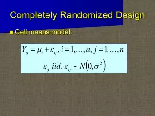
12. The model for the response is: • Yi,j = m + Ti + random error • with • Yi,j being any observation for which X1 = i • (i and j denote the level of the factor and the replication • within the level of the factor, respectively) • (or mu) is the general location parameter • Ti is the effect of having treatment level i

13. Experiment That same pharmaceutical company as before would like to examine the potency of a liquid medication mixed in large vats. To do this, a random sample of 5 vats from a month’s production was obtained, and 4 separate samples were selected from each vat. In total we have 4 x 5 or 20 pieces of data. We want to see if there is a significant difference between the five vats, that is, if: H0: T1 = T2 = T3 = T4 = T5 = 0 vs. Ha: At least one different from 0

14. Data from last month’s production

15. To analyze the data, we will run an Analysis of Variance (ANOVA). The ANOVA will separate out the variation due to random error within the treatment groups and any possible variation due to differences in the treatments – in this case, any variation between the average response for each vat. Estimate for m  in our model is the average of all the data (Ybar). Estimate for Ti :    Yi bar – Y-bar

16. ANOVA Table SourcedfSum of Sq.Mean Square Treatments t-1 SST SST/(t-1) Withint(r-1)SSWSSW/(t(r-1)) Total tr-1 SST

20. The Box Plot is a graphical display that provides important quantitative information about a data set. Some of this information is Location or central tendency Spread or variability Departure from symmetry Identification of “outliers” The Box Plot

21. A box plot or boxplot (also known as a box-and-whisker diagram or plot) is a convenient way of graphically depicting groups of numerical data through their five-number summaries: the smallest observation (minimum), lower quartile (Q1), median (Q2), upper quartile (Q3), and largest observation (maximum). A boxplot may also indicate which observations, if any, might be considered outliers. More information of Box Plots

23. Fisher’s LSD (Least Significant Difference) • Fisher’s LSD is a method for comparing treatment group means after the ANOVA null hypothesis of equal means has been rejected using the ANOVA F-test. If the F-test fails to reject the null hypothesis this procedure should not be used. • At this point we are interested in doing pairwise comparisons of the means. That is, we want to test hypotheses of the sort H0 : μ1 = μ2, H0 : μ1 = μ3, etc. The LSD method for testing the hypothesis • H0 : μ1 = μ2 proceeds as follows: • Calculate LSD1,2 = t0.05/2,DFW SQRT[MSW(1/n1 + 1/n2)] • where DFW = DF(within) and MSW = MS(within).

24. 2. If |y-bar1 − y-bar2| > LSD1,2 then we reject the null hypothesis H0 : μ1 = μ2. We then continue to test all pairs of interest. In this case the LSD is the same for all pairs because n1 = n2 = n3 = n4 = n5. More Information of LSD Method Another method that can be used is called the Tukey-Kramer Method. For information on that, then select the following link: Tukey-Kramer Method

25. So let’s see what our results are based on the Fisher’s Least Significant Difference procedure.LSD = 2.131 x SQRT[.0918 x (1/4 +1/4)] with DFW = 15 is 0.461 vs. 2: 0.8 2 vs. 3: 0.85 3 vs. 4: 0.851 vs. 3: 0.05 2 vs. 4: 1.7 3 vs. 5: 1.41 vs. 4: 0.9 2 vs. 5: 0.55 4 vs. 5: 2.251 vs. 5: 1.35

26. Conclusion: Reject H0 that the Vat’s all have the same potency at the 95% confidence level. Also, Vats #1 & #3 appear to have the same potency, while #2, #4 and #5 differ with Vat #1. Vat #3 differs from Vats #2, #4 and #5 in terms of potency. Vat #2, #4 and #5 are different from each other. #5 #2 #1 #3 #4

27. Randomized Block Design • Blocking is grouping experimental units that have similar effects on the response variable. • Successful blocking minimizes the variation among the experimental units within a block while maximizing the variation between the blocks. • Differences between blocks can be eliminated from the experimental error, thereby increasing the precision of the experiment. • Precision usually decreases as the block size increases.