Download
1 / 15
150 likes | 454 Views
Decomposition nonstationary turbulence velocity in open channel flow. Ying-Tien Lin 2005.12.12. Background. Laminar flow and turbulent flow. Background. Flow velocity profile. Turbulent velocity or Fluctuated velocity. Mean velocity. Background. Turbulent flow occurs in our daily life.

E N D
Decomposition nonstationary turbulence velocity in open channel flow Ying-Tien Lin 2005.12.12
Background • Laminar flow and turbulent flow
Background • Flow velocity profile
Turbulent velocity or Fluctuated velocity Mean velocity Background • Turbulent flow occurs in our daily life. put cube sugar into a cup of coffee • Turbulent model Assume
Background • Reynolds shear stress Sediment particles Shear stress River
Background • Stationary turbulence flow • Nonstationary turbulence flow (occurs in flooding period) Mean velocity How to find its time-varying mean velocity?
Decomposition method • Fourier decomposition method • Wavelet transformation • Empirical mode decomposition
Fourier decomposition method • It is unable to show how the frequencies vary with time in the spectrum. DFT LF Inv. DFT
Wavelet transformation • Linear combinations of small wave • Be able to show the frequency varies with time DWT Threshold Inv. DWT
Empirical Mode Decomposition (EMD) • The upper and lower envelopes of U(t) are constructed by connecting its local maxima and minima. Upper envelope Velocity Instantaneous velocity Lower envelope Time
Empirical mode decomposition (EMD) • The mean value of the two envelopes is then computed. The difference between the instantaneous velocity and the mean value is called the first intrinsic mode function (IMF), c1(t). IMF is a function that: 1. has only one extreme between zero crossings. 2. has a mean value of zero. This is called the Sifting Process
C1(t) C5(t) C12(t) residual(t)
Results Add noise Denoising
Results Add noise Denoising
Summary • These three decomposition methods perform good fitting with the original functions. • EMD seems better than the other two methods.