Workshop on Algorithm Implementation within the Aquarius Data Processing System 21-22 March 2007
College of Engineering Department of Atmospheric, Oceanic & Space Sciences. Workshop on Algorithm Implementation within the Aquarius Data Processing System 21-22 March 2007. Aquarius Radiometer RFI Flag. Chris Ruf Space Physics Research Laboratory

Workshop on Algorithm Implementation within the Aquarius Data Processing System 21-22 March 2007
E N D
Presentation Transcript
College of Engineering Department of Atmospheric, Oceanic & Space Sciences Workshop on Algorithm Implementation within the Aquarius Data Processing System 21-22 March 2007 Aquarius RadiometerRFI Flag Chris Ruf Space Physics Research Laboratory Dept. of Atmospheric, Oceanic & Space Sciences University of Michigan cruf@umich.edu, 734-764-6561 (V), 734-936-0503 (F)
Outline • Description of RFI Flag Algorithm • Demonstration of performance using JPL-PALS measurements with data sampling conditions similar to Aquarius in-flight • Algorithm Input Data and Configuration Parameters and Processed Outputs • Back Up Slides • Sensitivity of False Alarm Rate and Probability of Missed Detection to parameters of the algorithm • Description and demonstration of new kurtosis-based RFI detection method
Qualitative Description of Algorithm • The RFI detection algorithm is a “glitch detector” which identifies samples that deviate anomalously from the average of their neighbors • Adjustable parameters of the algorithm address • How many neighboring samples to use to determine the local average • Which neighboring samples to exclude from the average due to possible RFI contamination • How large a deviation from the local average constitutes the presence of RFI • Which (if any) other samples near a contaminated sample should also be flagged as contaminated even if they are not flagged directly by the algorithm
Relevant Aquarius Data Sampling Parameters • Calibrated TB samples are measured every 10ms • Satellite ground track velocity is ~ 7.5km/s • Radiometer HPBW footprint diameters are ~ 85, 102 and 125 km • Derived relationships • A very sharp TB feature, such as a coastal crossing, requires approximately 13 seconds (= HPBW/vgroundtrack) to develop in the Aquarius image • There will be approximately 1300 TB samples taken during a coastal crossing transition • Concern: Possible RFI false alarms during the most rapid changes in TB (e.g. at coastal crossings)
Description of Algorithm, pg 1 of 2 • Step 1: Determine local mean TB at sample under test • Step 1a: Compute dirty local mean, denoted by <TB1> • Average WS TB samples within +/- WS/2 of sample under test • Do not include the sample under test in the average • Step 1b: Identify dirty TBi samples among the WS samples • Sample TBi is dirty if (TBi - <TB1>) > TmDT • Tm is the mean threshold, an adjustable parameter of the algorithm • DT, the t=10 ms radiometer NEDT, is a fixed variable of the algorithm • Step 1c: Re-compute local mean without dirty samples, denoted by <TB>
Description of Algorithm, pg 2 of 2 • Step 2: Decide if the sample under test is corrupted by RFI • Sample under test is flagged as corrupted if • (TBunder test - <TB>) > TdetDT • Tdet is the detection threshold, an adjustable parameter of the algorithm • DT, the t=10 ms radiometer NEDT, is a fixed variable of the algorithm • Step 3: Also flag nearby samples as corrupted because they may be corrupted at a level below the detection threshold • Flag all samples within +/- Wr,f of the sample under test • Wr.f is an adjustable parameter of the algorithm (possibly= 0)
Dependence of Algorithm on its Parameters • Characterize algorithm performance using • False Alarm Rate (identifying RFI when there isn’t any) • Probability of Missed Detection (missing the identification of RFI that is present) • Use ground based L-Band PALS measurements made during April-May 2006 at JPL with JPL-PALS RF front end and University of Michigan Agile Digital Detector back end • ADD measures the 1st – 4th moments of the pre-detection signal • The 2nd moment is a traditional square law detector • The kurtosis is derived from 2nd and 4th central moments • Reliably identifies RFI with power levels at or above the radiometer NEDT
Description of PALS Data Sets Used, pg 1 of 4 • Data Set B: Nadir sky view with no RFI present • 2nd moment time series shown • Clear of RFI; variations almost exclusively due to NEDT
Description of PALS Data Sets Used, pg 2 of 4 • Data Set C: Nadir sky view with strong RFI present • 2nd moment time series shown • Large TB spikes typical of weekday daytime RFI near Bldg. 168
Description of PALS Data Sets Used, pg 3 of 4 • Data Set D: Nadir sky to absorber transition with no RFI • 2nd moment time series shown; elapsed time from cold sky to ambient BB absorber (13 sec) is approximately the same as Aquarius costal crossing transition
Description of PALS Data Sets Used, pg 4 of 4 • Data Set E: Nadir sky to absorber transition with artificial RFI added • 2nd moment time series shown; RFI added at approximate location of coastline
Example #1 of Algorithm Performance • Data Set C (nadir sky w/ RFI) • Algorithm parameters: Ws=20, Tm=1.5, Tdet=4, Wr=Wf=5 • Several missed detections (bottom plot) near t = 6 and 10 seconds
Example #2 of Algorithm Performance • Data Set D (simulated coastal crossing w/ no RFI) • Algorithm parameters: Ws=20, Tm=1.5, Tdet=4, Wr=Wf=5 • False alarms more likely near coastal crossing
Example #3 of Algorithm Performance • Data Set E (simulated coastal crossing w/ single RFI event at coastline) • Algorithm parameters: Ws=20, Tm=1.5, Tdet=4, Wr=Wf=5 • Single RFI event successfully detected; false alarms still present
Algorithm Input Data • Samples of the raw (shortest integration time; either 0.01 s or 0.02 s) radiometer antenna counts, CANT • For each sample to be tested for RFI, the preceding and subsequent 30 CANT samples from the same radiometer at the same polarization are also needed • Time tag for each CANT sample • For each sample, a time tag is needed from which the relative time between each of the 61 samples can be determined. • The time can be referenced to any common point in the integration interval (e.g. any of the start time, the center time or the end time of the integrator is okay) • Location (latitude, longitude) of the center of the radiometer antenna footprint for the CANT sample under test • Precision: Rounded to nearest 1 deg
Algorithm Input Configuration Parameters • Local mean running average window, WM • Values for this parameter are assigned independently in 1 degree increments of latitude and longitude and for each of the three radiometers. Units: seconds; Resolution: 0.001 s • Local mean running average glitch threshold, TM • Values for this parameter are assigned independently in 1 degree increments of latitude and longitude and for each of the three radiometers. Units: unitless; Resolution: 0.01 • RFI detection glitch threshold, TD • Values for this parameter are assigned independently in 1 degree increments of latitude and longitude and for each of the three radiometers. Units: unitless; Resolution: 0.01 • RFI detection neighborhood window, WD • Values for this parameter are assigned independently in 1 degree increments of latitude and longitude and for each of the three radiometers. Units: seconds; Required resolution: 0.001 s • Nominal standard deviation of radiometer antenna counts, STDANT • Values for this parameter are assigned independently for each of the three radiometers. Units: radiometer counts; Required resolution: 0.01 counts
Algorithm Processed Ouputs • Number of CANT samples in the neighborhood of the sample under test (neighborhood as defined by WM) that were flagged with RFI • Resolution: integer value between 0 and 60 • Number of standard deviations that the sample under test deviated from the local mean by • Resolution: one significant digit, i.e. xx.1. • RFI detection word • =3 if RFI detected in sample under test and in neighbors • =2 if RFI detected in sample under test only • =1 if RFI detected in neighbors only • =0 if RFI not detected in sample under test or in neighbors
WS and Tm Affects on False Alarm Rate, pg 1 of 2 • Vary local averaging window (WS) and mean threshold (Tm) • Evaluate False Alarm Rate using Data Set B (clean sky view) • WS has little effect; FAR varies inversely with Tm as expected
WS and Tm Affects on False Alarm Rate, pg 2 of 2 • Vary local averaging window (WS) and mean threshold (Tm) • Evaluate False Alarm Rate using Data Set C (clean simulated coastal crossing) • WS has little effect; FAR varies inversely with Tm but with significantly higher values (approximately double) as compared to constant TB sky view
WS Affect on Missed Detections, pg 2 of 2 • Single coastal-crossing RFI event not missed • ~44% of RFI events in Data Set C (nadir sky w/ strong RFI) missed • Missed detection rate is not dependent on WS
Wr,f Affect on False Alarm Rate • Vary window of otherwise clean neighboring samples flagged with RFI (Wr,f) • Evaluate False Alarm Rate using Data Set B (clean sky view) • Increasing Wr,f increases FAR as expected, since no RFI is actually present
Wr,f Affect on Missed Detections • Vary window of otherwise clean neighboring samples flagged with RFI (Wr,f) • Evaluate Missed Detections using Data Sets C,D,E (nadir sky w/ RFI and coastal crossings) • Increasing Wr,f decreases missed detections for Data Set C; no detections missed for coastal crossing data sets
Tm and Tdet Affect on False Alarm Rate, pg 1 of 2 • Vary mean threshold (Tm) and detection threshold (Tdet) • Evaluate False Alarm Rate using Data Set B (clean sky view) • Lowering either Tm or Tdet will increase the FAR
Tm and Tdet Affect on False Alarm Rate, pg 2 of 2 • Vary Tm and Tdet and evaluate False Alarm Rate as in previous slide • Plot with Tdet on x-axis; Tdet has largest effect on FAR of any parameter
Tdet Affect on Missed Detections • Vary Tdet and evaluate missed detections using Data Sets C,D,E (nadir sky w/ RFI and coastal crossings) • Decreasing Tdet decreases missed detections for Data Set C; no detections missed for coastal crossing data sets
College of Engineering Department of Atmospheric, Oceanic & Space Sciences Agile Digital DetectorforRFI Mitigation mRad 2006 9th Specialist Meeting on Microwave Radiometry and Remote Sensing Applications San Juan, Puerto Rico 28 February – 3 March 2006 Chris Ruf, Sidharth Misra & Roger De Roo Dept. of Atmospheric, Oceanic & Space Sciences University of Michigan cruf@umich.edu, 734-764-6561 (V), 734-936-0503 (F)
Outline • Objectives • Develop a way to detect and mitigate Radio Frequency Interference that can reliably differentiate between low level RFI and the natural geophysical variability of brightness temperature • Assess the technological feasibility of implementing the approach on a spaceborne microwave radiometer • Agile Digital Detector Theory of Operation • Prototype Design • Field Tests
Agile Digital Detector (ADD)Theory of Operation • Conventional microwave radiometer square law detectors measure the 2nd moment of the noise voltage • ADD measures either: a) the probability density function; or b) select higher order moments of the noise voltage • Non-gaussian distributed RFI can be detected • Digital sub-banding permits mitigation filtering • Very low level RFI can be reliably discriminated from natural variability in brightness temperature
Approaches to Detecting RFI • Time domain – look for pulses • Frequency domain – look for carrier frequencies • Amplitude domain – look for non-thermal distribution • Correlation domain – e.g. Look for polarization signatures Gaussian pdf Thermal waveform Sinusoidal waveform Non-Gaussian pdf
RFI Detection Using Higher Order Moments • The kurtosis of a random variable, x, is defined as • k=3 for a gaussian distributed r.v., independent of sx2 (i.e. k=3 for gaussian thermal noise, independent of TB) • The standard deviation of an estimate of k after a finite integration time is • For prototype radiometer operation (B=3 MHz & t=0.3 s), Dk = 0.005 • RFI Detection Flag if |k – 3| > 3Dk
L-Band ADD Prototype Functional Block Diagram • High speed ADC followed by 8 x 3 MHz subbands cover 1401.5-1425.5 MHz • 128 level discrete probability density function at each level • Parallel V- and H-pol channels + 3rd Stokes digital cross-correlation
Demonstration Tests • Installed in ground based L-Band radiometer • May ’05: Artificial radar pulses added to LN2 BB Load • Jun ’05: Field deployment near ARSR-1 air traffic control radar • Installed in NOAA/ETL PSR C-Band Stepped LO channel • Aug ’05: Airborne flight over Houston/Dallas/San Antonio/Gulf of Mexico • data analysis still in progress
ADD Prototype Installed in Ground based L-Band Radiometer • Truck mounted fully polarimetric L-Band radiometer operated by the U-M Microwave Geophysics Lab • Deployed in Canton, MI at ARSR-1 air traffic control radar site in June 2005 • Collaborators: J. Piepmeier (NASA GSFC) and J. Johnson (OSU) concurrently operated other RFI mitigation back ends
Outdoor Sky Cal with sinusoidal RFI8 Subband Probability Density Functions • TB = 40 K plus ~260 K sine wave injected into subband 5
LN2 Load Cal with pulsed sinusoidal RFI60s time series of kurtosis/3 in 8 subbands • Normalized kurtosis is 1.000 +/- 0.002 in subbands 1-2,6-8 • Normalized kurtosis is 1.007 in subbands 3&5; 2.35 in subband 4
Near ARSR-1 Air Traffic Control RadarCanton, MI (N42 16' 36", W083 28' 27") Transmits at ~1305 MHz / Peak transmit power 4 MW / Pulse width 2 ms / Pulse repetition frequency 360 Hz / Azimuth scan 10 sec per revolution.
Near ARSR-1 Air Traffic Control Radar60s time series of <x4>/<x2>2/3 in 8 subbands • Antenna pointing at tree line away from radar; RFI from bi-static ground clutter • 10s azimuth scan period evident in subband 1 • Strong non-gaussian kurtosis in subbands 4&5
Near ARSR-1 Air Traffic Control Radar60s time series of RFI-corrected TB • Row 1: TB using all 8 subbands • Row 2: TB using only subbands with normalized kurtosis within 3s of 1.000 • Row 3: TB difference between rows 1&2 (RFI level of 0-1K) • Row 4: # of RFI-free subbands
Numerical simulation – Dependence of Kurtosis on strength of pulsed sinusoidal RFI • (a) 1% duty cycle and variable amplitude • (b) 10% duty cycle and variable amplitude • (c) 100% duty cycle (i.e. continuous wave) and variable amplitude • (d) fixed amplitude and variable duty cycle. SNR is the ratio between the variance of the sinusoid and of the gaussian noise signal, which corresponds to the relative brightness temperature of the RFI and the earth scene.
Example of PSR Flight DataKurtosis and 2nd Moment Spectra • Kurtosis (left) and 2nd moment (below) 5.5-7.5 GHz spectra v. time over Dallas Metro area • ch = 50-80 (~6 GHz), intermittent times • Strong non-gaussian kurtosis • Strong, correlated effect on TB • ch = 170-180 (~7.5 GHz), t = 0-60s • Strong non-gaussian kurtosis • Not so noticeable effect on TB
Closer Look at PSR Flight Data – RFI with Strong TB Kurtosis (left) and 2nd moment (right) spectra near 6 GHz v. time over Dallas Metro area
Closer Look at PSR Flight Data – RFI with Weak TB Kurtosis (left) and 2nd moment (right) spectra near 7.5 GHz v. time over Dallas Metro area
Performance Summary • Direct measurement of PDF can be used to reliably detect non-gaussian RFI • Experimental verification of Dkurtosis noise floor • sk = 0.002 is consistent with [24/(Bt)]1/2 theory • 3s deviation is exceeded with RFI level ~ NEDT • Digital subbands allow RFI to be removed