Supply: Production

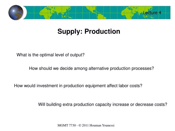
Supply: Production What is the optimal level of output? How should we decide among alternative production processes? How would investment in production equipment affect labor costs? Will building extra production capacity increase or decrease costs?

Supply: Production Quantity(widgets) 1500 Total Output 1200 900 600 300 Labor 3 6 9 12 15

Quantity(widgets) 1500 B Total Output 1200 900 A 600 300 Labor 3 6 9 12 15

Average and Marginal output (product) curves B 170 A 150 130 110 90 Average Output (Average Product) Q/L 70 50 30 C 10 -10 1 2 3 4 5 6 7 8 9 10 11 12 13 14 15 16 -30 Marginal OutPut (Marginal Product) dQ/dL -50

Average output (product) or in general Where X is a given input into production Average output is either zero or positive Maximum Average output Point A is precisely that: the point where average output is at its highest.

Marginal output (product) Where X is a given input into production A measure of productivity, it measures the rate of change of output (production) as an extra unit of input is added. A production reaches maximum productivity with respect to a given input (assuming all other inputs are constant) when marginal output for that particular input is maximized (Point B) .

Marginal output (product) The difference between and Assumes continuous units (e.g. labor in labor-hours 2.73 units is allowed) 1500 1200 900 Assumes discrete units (e.g. labor in persons n or n+1 but not 1.5n) 600 300 3 6 9 12 15

Marginal output (product) As expected, output is maximized when marginal output (marginal product) is zero (point C). In general Output = Q(L,M,N,X,Y,Z,…) In our simple case Output=Q(L) As such:

Marginal output (product) Exercise: Show that in all cases, average output is maximum when marginal output is equal to it. e.g. point A Average product (average output) is Maximum average product (average output) is when its derivative is equal to zero Average product is zero when:

The Law of Diminishing Marginal Returns If equal increments of an input are added whilst at least one other input is held constant, there is a point beyond which the resulting product output would start to decrease. Note: • This is an empirical generalization and not a law of nature • It is assumed that production technology does not change Example: Adding staff but not workstations

Optimal Resource Utilization How much of a resource (input variable) should a firm use? What do want to maximize: ? • Output • Revenue • Profit C Correct answer is:

Optimal Resource Utilization Marginal Revenue Product (MRP) is the amount that an additional unit of the variable input adds to the firm’s total revenue (i.e. if MRPY is the marginal revenue product of input Y): However note that : As such: Therefore: The marginal revenue product of an input equals to that input’s marginal product times the firm’s marginal revenue

Optimal Resource Utilization Similarly: Marginal Product Expenditure (MPE) is the amount that an additional unit of the variable input adds to the firm’s total costs (i.e. if MPEY is the marginal product expenditure of input Y): However note that : As such: Therefore: The marginal product expenditure of an input equals to that input’s marginal product times the firm’s marginal cost

Optimal Resource Utilization To maximize profit (globally): or: Multiplying both sides by: Rearranging:

Optimal Resource Utilization Example: A brewery has fixed plant and equipment. The output of this brewery is shown to relate to its labor usage according to the following equation where L is the number of workers hired per day and Q is the quantity of beer produced. This is a thirsty country and the brewery can sell all the beer it can produce for $20 a gallon. This is also a developing country so the brewery can hire as many workers as it needs for $40 a day. How many workers should the brewery hire?

Optimal Resource Utilization The brewery's marginal revenue is MR= $20 The brewery's marginal product expenditure is MPEL= $40 Marginal product for labor is: Marginal revenue product for labor is: To maximize, we must have:

Multi-variable Production Functions A production function is very rarely a function of only one variable. For example Q may be a function of: Where L stands for cost of Labor, M stands for cost of Machinery and T stands for cost of Transportation In most cases – certainly all cases covered in this course - the mathematics and formulations are exactly the same as for the case of a single variable instance except that we assume – in turn – that all other variables except the one of our interest are constants. We also use the partial differential notation to indicate multi-variability.

Multi-variable Production Functions Example: Our brewery has the production function: How much should they spend on transportation if it costs $200 to transport one gallon of beer?

Isoquants: Choosing Combinations of Inputs What are the possible combinations of various inputs that are capable of producing a certain quantity of output? Capital Capital/Labor Isoquants 50 A 40 30 B 20 300 C 200 10 100 7 Labor 1 2 3 4 5 6

Marginal Rate of Substitution The rate at which one input can be substituted for another in such a way that the output remains constant Change in one input Change in another input Rate of change of one over the other input At the limit

Marginal Rate of Substitution Exercise: Show that the marginal rate of substitution is equal to the ratio of the marginal output (marginal product) of the inputs concerned. By definition: Therefore:

Isoquants: Choosing Combinations of Inputs Isoquants may have regions of positive slope! These are regions where the quantities of BOTH inputs must increase in order to maintain a fixed level of production. For the slope of an isoquant to be positive, it means that the marginal product of one or the other of the inputs must be negative. This is not efficient! As such we restrict ourselves to operating within the range where the slope of the isoquants are negative. Such region is called the Economic Region of Production

Economic Region of Production Economic Region of Production Capital 50 300 40 30 200 20 100 10 7 1 2 3 4 5 6 Labor

Isocosts: Choosing Combinations of Inputs What combinations of inputs can we obtain for the same expenditure? In a two input situation, this is very simple, for a fixed outlay (e.g. of money), we will have: Where X and Y represent the amount of each input respectively, and PX and PY represent the unit cost for each unit of each input. Rewriting this we get: Which is the equation for a straight line called the isocost line of X and Y

Isocosts: Choosing Combinations of Inputs Y K/PY Slope = -PX/PY K/PX X

Choosing Combinations of Inputs What point on the isocost line would you pick? Y K/PY Q K/PX X Pick the point that lies on both the isocost curve and the highest isoquant

Choosing Combinations of Inputs Analytically: The Q point that optimizes the input combinations is the point where the isocost line is a tangent to the isoquant. We know that the slope of the isocost line is: We also know that the slope of the isoquant curve (at a given point) is: Therefore the Q point is where the slope of the isocost curve equals the ratio of the marginal products: In fact in general when more than two inputs are involved:

Example: An automobile manufacturer has determined that the quantity of automobiles they manufacture relates to the number (in thousands) of factory workers (F) and the number (in thousands) of office workers (O): The monthly salary for an office worker is $4000 and the monthly wage for a factory worker is $2000. how many office workers and how many factory workers should the company hire if they have allotted $2,600,000 a month to wages?

and that We know that: We calculate the marginal products: Substituting: Therefore: And as such:

Example: ABCO has a production equation as follows: Q is the output, L is the number of workers and K is the number of machines. The wages of a worker is $8 per hour and the price of a machine is $2 per hour. If ABCO produces 80 units of output per hour, how many workers and machines should it use? Again: and

then: so if: and therefore: as Q=80

Optimum Lot Size It is often more economical to produce items in lots. This is because doing so would reduce set up time for equipment and project start-up costs. For example if it costs S dollars to set up a machine to produce widgets and each widget manufacture cost is W, then if we produce 100 widgets we will have a total cost of manufacture per widget of: (S+100W)/100 If we produce 1000,000 widgets, then the manufacturing cost per unit will be (S+1000,000W)/1000000 So, it would pay to have as large a run as possible. However, things are not as easy. There is a force acting against us

Optimum Lot Size We have to carry all those widgets in inventory until we need them, which will cost money. Let us say the cost of carrying a widget in inventory is B. What should be our production lot size to minimize costs? We know that total set up cost equals SQ/L where S is the set up cost, Q is the quantity required, and L is the number of widgets produced in a given run. We also know that the cost of holding an item in inventory is B, as such the average cost of holding inventory is BL/2. We wish to find the optimum size of L that minimizes the total cost of

Optimum Lot Size We need to find a formula for cost. Therefore: To minimize:

Output Elasticity and Scalability What would happen to output quantity if we doubled all inputs? • It would double • It would less than double • It would more than double Answer: IT DEPENDS

Output Elasticity and Scalability It depends on a measure called output elasticity. Output elasticity is the measure of percent change in output resulting from a one percent increase in ALL inputs. Given a quantity Q say of X and Y, that is Q(X,Y), calculate Q’(1.01X+1.01Y) If : Then the production has constant return to scale Then the production has increasing return to scale Then the production has decreasing return to scale

Supply: Production