Download
1 / 26
260 likes | 269 Views
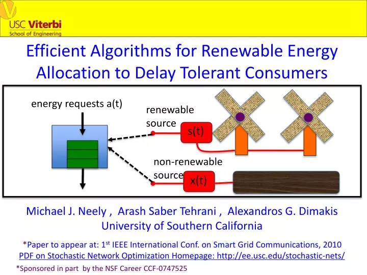
Efficient Algorithms for Renewable Energy Allocation to Delay Tolerant Consumers. energy requests a(t). renewable source. s(t). non-renewable source. x(t). Michael J. Neely , Arash Saber Tehrani , Alexandros G. Dimakis University of Southern California

E N D
Efficient Algorithms for Renewable Energy Allocation to Delay Tolerant Consumers energy requests a(t) renewable source s(t) non-renewable source x(t) Michael J. Neely , Arash Saber Tehrani , Alexandros G. Dimakis University of Southern California *Paper to appear at: 1st IEEE International Conf. on Smart Grid Communications, 2010 PDF on Stochastic Network Optimization Homepage: http://ee.usc.edu/stochastic-nets/ *Sponsored in part by the NSF Career CCF-0747525
energy requests a(t) renewable source s(t) non-renewable source • Renewable sources of energy can have variable and unpredictable supplies s(t). • We can integrate renewable sources more easily if consumers tolerate service within some maximum allowable delay Dmax. • Might sometimes need to purchase energy from non-renewable source to meet the deadlines, and purchase price can be highly variable.
Example Data: (Top Row) Spot Market Price (Bottom Row) Energy Production in a California Wind Turbine Electricity Price ($) Energy Production (MW/h)
a(t) Renewable source s(t) Non-Renewable source x(t), γ(t) Talk Outline: • First Problem: Minimize time average cost of purchasing non-renewable energy (i.i.d. case) • Second Problem: Joint pricing of customers and purchasing of non-renewables (i.i.d. case). • Generalize to arbitrary sample paths using “Universal Scheduling Theory” of Lyapunov Optimization. • Simulation results using CAISO spot market prices γ(t) and 10-minute energy production s(t)from Western Wind resources Dataset (from National Renewable Energy Lab).
Problem 1: Minimize Average Cost of Non-Renewable Purchases a(t) Renewable source s(t) Non-Renewable source x(t), γ(t) • Slotted Time: t = {0, 1, 2, …} • a(t) = energy requests on slot t (serve with max delay Dmax). • s(t) = renewable energy supply on slot t. (“use-it-or-loose-it”) • x(t) = amount non-renewable energy purchased on slot t. • γ(t) = $$/unit energy price of non-renewables on slot t. • Q(t) = Energy request queue requests (random) Q(t+1) = max[Q(t) – s(t) – x(t), 0] + a(t) , cost(t) = x(t)γ(t) purchase price (random) Renewable supply (random) (use-it-or-loose-it) Non-Renewables purchased (decision variable)
Problem 1: Minimize Average Cost of Non-Renewable Purchases a(t) Renewable source s(t) Non-Renewable source x(t), γ(t) Q(t+1) = max[Q(t) – s(t) – x(t), 0] + a(t) , cost(t) = x(t)γ(t) • Assumptions: • For all slots t we have: • 0 ≤ a(t) ≤ amax , 0 ≤ s(t) ≤ smax , 0 ≤ γ(t) ≤ γmax, 0 ≤ x(t) ≤ xmax • xmax units of energy always available for purchase from • non-renewable (but at variable price γ(t)). • amax≤ xmax (possible to meet all demands in 1 slot at high cost) • (a(t), s(t), γ(t)) vector is i.i.d. over slots with unknown distribution
Problem 1: Minimize Average Cost of Non-Renewable Purchases Q(t+1) = max[Q(t) – s(t) – x(t), 0] + a(t) , cost(t) = x(t)γ(t) • Possible formulation via Dynamic Programming (DP): • “Minimize average cost subject to max-delay Dmax.” • This can be written as a DP, but requires distribution knowledge. • Recent work on delay tolerant electricity consumers using DP is: • [Papavasiliou and Oren, 2010] • We will not use DP. We will take a different approach...
Problem 1: Minimize Average Cost of Non-Renewable Purchases Q(t+1) = max[Q(t) – s(t) – x(t), 0] + a(t) , cost(t) = x(t)γ(t) • Relaxed Formulation via Lyapunov Optimization for Queue Networks: • Minimize: E{cost} (time average) • Subject to: (1) E{Q} < infinity (a “queue stability” constraint) • (2) 0 ≤ x(t) ≤ xmax for all t • Define cost* = min cost subject to stability • By definition: cost* ≤ cost delivered by any other alg (including DP) • We will get within O(δ) of cost*, with worst-case delay of 1/δ. Avg. Cost our performance optimal DP Ο(δ) cost* Worst Case Delay
Advantages of Lyapunov Optimization for Queueing Networks: • No knowledge of distribution information is required. • Explicit [O(δ), O(1/δ)] performance guarantees. • Robust to changes in statistics, arbitrary correlations, non- ergodic, arbitrary sample paths (as we will show in this work). • Worst case delay bounds (as we will show in this work). • No curse of dimensionality: Implementation is just as easy in extended formulations with many dimensions: General Lyapunov Optimization Problem: [Georgiadis, Neely, Tassiulas, F&T 2006] Minimize : E{y} Subject to: (1) E{xi} ≤ 0 for all i in {1, …, N} (2) Queue k is stable for all k in {1, …, K} (3) Control action on slot t in ActionSpace(t) (for all t in {0, 1, 2, …} )
Virtual Queue for Worst-Case Delay Guarantee (fix ε>0): s(t)+x(t) a(t) Actual Queue Q(t) Virtual Queue (enforces ε-persistent service) ε1{Q(t)>0} s(t)+x(t) Z(t) Z(t+1) = max[Z(t) – s(t) – x(t) + ε1{Q(t)>0}, 0] Theorem: Any algorithm with bounded queues Q(t) ≤ Qmax, Z(t) ≤Zmax for all t yields worst-case delay of: Dmax = Qmax + Zmax slots ε Proof Sketch: Suppose not. Consider slot t, a(t): t +Dmax a(t) [s(τ)+x(τ)] ≤ Qmax Then: Q(t) ≤ Qmax τ=t Implies: Z(t+Dmax) > Zmax (contradiction) t t+Dmax
Stabilize Z(t) and Q(t) while minimizing average cost cost(t): Z(t) Lyapunov Function: L(t) = Z(t)2 + Q(t)2 Lyapunov Drift: Δ(t) = E{L(t+1) – L(t)|Z(t), Q(t)} Take actions to greedily minimize “Drift-Plus-Weighted-Penalty”: Minimize: Δ(t) + Vγ(t)x(t) where V is a postiive constant that affects the [O(1/V), O(V)] Cost-delay tradeoff. (using V=1/δ recovers the [O(δ), O(1/δ)] tradeoff.) Q(t)
Resulting Algorithm: Every slot t, observe (Z(t), Q(t), γ(t)). Then: • Choose x(t) = { 0 , if Q(t) + Z(t) ≤ Vγ(t) • { xmax, if Q(t) + Z(t) > Vγ(t) • Update virtual queues Q(t) and Z(t) according to their equations • Define: Qmax = Vγmax + amax , Zmax = Vγmax + ε • Theorem: Under the above algorithm: • Q(t) ≤ Qmax, Z(t) ≤ Zmax for all t. • Delay ≤ (Qmax + Zmax)/ε = O(V) • Further, if (s(t), a(t), γ(t)) i.i.d. over slots, and if ε≤ max[E{a(t)}, E{s(t)}] • Then: • E{cost} ≤ cost* + B/V • [where B = (smax + xmax) 2 + amax2 + ε2]
Problem 2: Joint Pricing and Energy Allocation E{a(t)} = F(p(t), y(t), γ(t)) Renewable source s(t) p(t) Non-Renewable source x(t), γ(t) • Same system model, with following extensions: • a(t) = arrivals = Random function of pricing decision p(t) • h(t) = additional “demand state” (e.g. “HIGH, MED, LOW”) • E{a(t)|p(t), h(t), γ(t)} = F(p(t), h(t), γ(t)) = Demand Function Example: h(t) = HIGH h(t) = MED F(p(t), h(t), γ(t)) Demand Function h(t) = LOW price p(t) γ(t)
Problem 2: Joint Pricing and Energy Allocation E{a(t)} = F(p(t), y(t), γ(t)) Renewable source s(t) p(t) Non-Renewable source x(t), γ(t) • Same system model, with following extensions: • a(t) = arrivals = Random function of pricing decision p(t) • h(t) = additional “demand state” (e.g. “HIGH, MED, LOW”) • E{a(t)|p(t), h(t), γ(t)} = F(p(t), h(t), γ(t)) = Demand Function • New Problem: • Profit(t) = a(t)p(t) – x(t)γ(t) • Maximize Time Average Profit! • Profit* = Optimal Time Avg. Profit Subject to Stability
Problem 2: Joint Pricing and Energy Allocation E{a(t)} = F(p(t), h(t), γ(t)) Renewable source s(t) p(t) Non-Renewable source x(t), γ(t) Drift-Plus-Penalty for New Problem: • Δ(t) – VE{Profit(t)|Z(t),Q(t)} = Δ(t) – VE{a(t)p(t) – x(t)γ(t)|Z(t),Q(t)} • Every slot t, observe (h(t), Z(t), Q(t),γ(t)). Then: • (Pricing) Choose p(t) in [0, pmax] to solve: • Maximize: F(p(t),h(t),γ(t))(Vp(t) – Q(t)) • Subject to: 0 ≤ p(t) ≤ pmax • (Purchasing) Choose x(t) same as before. • Update queues Q(t), Z(t) same as before. Resulting Algorithm:
Problem 2: Joint Pricing and Energy Allocation E{a(t)} = F(p(t), h(t), γ(t)) Renewable source s(t) p(t) Non-Renewable source x(t), γ(t) Drift-Plus-Penalty for New Problem: • Δ(t) – VE{Profit(t)|Z(t),Q(t)} = Δ(t) – VE{a(t)p(t) – x(t)γ(t)|Z(t),Q(t)} • Every slot t, observe (h(t), Z(t), Q(t),γ(t)). Then: • (Pricing) Choose p(t) in [0, pmax] to solve: • Maximize: F(p(t),h(t),γ(t))(Vp(t) – Q(t)) • Subject to: 0 ≤ p(t) ≤ pmax • (Purchasing) Choose x(t) same as before. • Update queues Q(t), Z(t) same as before. Resulting Algorithm: *If F(p,h,γ) = β(h)G(p,γ), don’t need to know demand state h(t)!
Problem 2: Joint Pricing and Energy Allocation E{a(t)} = F(p(t), h(t), γ(t)) Renewable source s(t) p(t) Non-Renewable source x(t), γ(t) Drift-Plus-Penalty for New Problem: • Δ(t) – VE{Profit(t)|Z(t),Q(t)} = Δ(t) – VE{a(t)p(t) – x(t)γ(t)|Z(t),Q(t)} • Every slot t, observe (h(t), Z(t), Q(t),γ(t)). Then: • (Pricing) Choose p(t) in [0, pmax] to solve: • Maximize: β(h(t))G(p(t),γ(t))(Vp(t) – Q(t)) • Subject to: 0 ≤ p(t) ≤ pmax • (Purchasing) Choose x(t) same as before. • Update queues Q(t), Z(t) same as before. Resulting Algorithm: *If F(p,h,γ) = β(h)G(p,γ), don’t need to know demand state h(t)!
Problem 2: Joint Pricing and Energy Allocation E{a(t)} = F(p(t), h(t), γ(t)) Renewable source s(t) p(t) Non-Renewable source x(t), γ(t) Theorem: Under the joint pricing and energy allocation algorithm: (a) Worst case queue bounds Qmax, Zmax same as before. (b) Worst case delay bound Dmax same as before, i.e., O(V). (c) If (s(t), γ(t), h(t)) i.i.d. over slots, and ε ≤ E{s(t)}, then: E{profit} ≥ profit* - O(1/V)
Universal Scheduling for Arbitrary Sample Paths… a(t) Renewable source s(t) Non-Renewable source x(t), γ(t) Consider the first problem again (x(t) = only decision variable): Suppose (s(t), γ(t), a(t)) have arbitrary sample path! (assumethey are still bounded: [0, smax], [0, γmax], [0, amax].) Universal Scheduling Theorem: (a) Worst case queue bounds Qmax, Zmax same as before. (b) Worst case delay bound Dmax same as before, i.e., O(V). (c) For any integers T>0, R>0: RT-1 R-1 1 1 x(t)γ(t) ≤ Cr* + BT/V RT R t=0 r=0 “Genie-Aided” T-Slot Lookahead Cost!
For every R>0, T>0: RT-1 R-1 1 1 x(t)γ(t) ≤ Cr* + BT/V RT R t=0 r=0 R frames of size T slots: … Frame 1 Frame 2 Frame 3 Frame R T-Slot Lookahead Problem for frame r in {0, …, R-1}: cr* computed below, assuming future values of (a(τ), s(τ), γ(τ)) are fully known in frame r:
Simulations over Real Data Sets: • We used 10 minute slot sizes (granularity of the available data) • Compare to simple “Purchase at Deadline” algorithm. • We chose V=100 Dmax = 400 slots (70 hours)
Same experiment: Histogram of Delay (V=100, ε= 87.5): Our algorithm yields worst-case delay considerably less than the bound Dmax. Worst case observed delay was 60 slots (10 hours)
Concluding Slide: a(t) Renewable source s(t) Non-Renewable source x(t), γ(t) • Lyapunov Optimization for Renewable Energy Allocation • No need to know distribution. Robust to arbitrary sample paths. • Explicit [O(1/V), O(V)] performance-delay tradeoff
Explanation of Why Delay is small even with ε=0… Even with ε=0, we still get the same Qmax bound. (Q(t) ≤ Qmax for all t). Delay of requests that arrive on slot t is equal to the smallest integer T such that: t +T [s(τ)+x(τ)] ≥ Q(t) τ=t So delay will be less than or equal to T whenever: t +T s(τ) ≥ Qmax τ=t There is no guarantee on how long this will take for arbitrary s(t) processes, but one can compute probabilities of exceeding a certain value if we try to use a stochastic model for s(t).