Download
1 / 40
420 likes | 874 Views
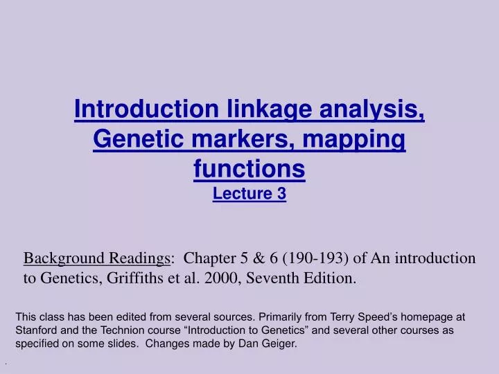
Introduction linkage analysis, Genetic markers, mapping functions Lecture 3. Background Readings : Chapter 5 & 6 (190-193) of An introduction to Genetics, Griffiths et al. 2000, Seventh Edition.

E N D
Introduction linkage analysis, Genetic markers, mapping functionsLecture 3 Background Readings: Chapter 5 & 6 (190-193) of An introduction to Genetics, Griffiths et al. 2000, Seventh Edition. This class has been edited from several sources. Primarily from Terry Speed’s homepage at Stanford and the Technion course “Introduction to Genetics” and several other courses as specified on some slides. Changes made by Dan Geiger. .
Purpose of human linkage analysisTo obtain a crude chromosomal location of the gene or genes associated with a phenotype of interest, e.g. a genetic disease or an important quantitative trait.Examples: Cystic fibrosis (found), Diabetes, Alzheimer, and Blood pressure.
LinkageStrategies I Traditional (from the 1980s or earlier) • Linkage analysis on pedigrees • Association studies: candidate genes • Allele-sharing methods: Affected siblings • Animal models: identifying candidate genes • Cell – hybrids Newer (from the 1990s) • Focus on special populations (Finland, Hutterites) • Haplotype-sharing (many variants)
Linkage Strategies II On the horizon (here) • Single-nucleotide polymorphism (SNPs) • Functional analyses: finding candidate genes Needed (starting to happen) • New multilocus analysis techniques, especially • Ways of dealing with large pedigrees • Better phenotypes: ones closer to gene products • Large collaborations
Horses for courses • Each of these strategies has its domain of applicability • Each of them has a different theoretical basis and method of analysis • Which is appropriate for mapping genes for a disease of interest depends on a number of matters, most importantly the disease, and the population from which the sample comes.
The disease matters Definition (phenotype), prevalence, features such as age at onset Genetics: nature of genes (Penetrance), number of genes, nature of their contributions (additive, interacting), size of effect Other relevant variables: Sex, obesity, etc. Genotype-by-environment interactions: Exposure to sun.
The population matters History: pattern of growth, immigration Composition: homogeneous or melting pot, or in between Mating patterns: family sizes, mate choice Frequencies of disease-related alleles, and of marker alleles Ages of disease-related alleles
106 years 105 years Immigration
Complex traits Definition vague, but usually thought of as having multiple, possibly interacting loci, with unknown penetrances; and phenocopies. Affected only methods are widely used. The jury is still out on which, if any will succeed. Few success stories so far. Important: heart disease, cancer susceptibility, diabetes, …are all “complex” traits. We focus more on simple traits where success has been demonstrated very often. About 6-8 percent of human diseases are thought o be simple Mendelian diseases.
Design of gene mapping studies How good are your data implying a genetic component to your trait? Can you estimate the size of the genetic component? Have you got, or will you eventually have enough of the right sort of data to have a good chance of getting a definitive result? Power studies. Simulations.
Genotyping A person is said to be typed if its markers have been genotyped. Choice of markers: highly polymorphic preferred. Heterozygosity and polymorphism information content (PIC)value are measures commonly used. Reliability of markers important too Good quality data critical: errors can play a surprisingly large role.
Preparing genotype data for analysis Data cleaning is the big issue here. Need much ancillary data…how good is it?
Analysis A very large range of methods/programs are available. Effort to understand their theory will pay off in leading to the right choice of analysis tools. Trying everything is not recommended, but not uncommon. Many opportunities for innovation.
Interpretation of results of analysis An important issue here is whether you have established linkage. The standards seem to be getting increasingly stringent. What p-value or LOD should you use? Dealing with multiple testing, especially in the context of genome scans and the use of multiple models and multiple phenotypes, is one of the big issues. E.g., Bonferroni correction.
References Related topics (not covered in this course): Exclusion mapping, homozygosity mapping, variance component methods, twin studies, and much more. Some of these topics plus others are covered in two books: Handbook of Human Genetic Linkageby J.D. Terwilliger & J. Ott (1994) Johns Hopkins University Press. Ordered, not available at the library. Analysis of Human Genetic Linkageby J. Ott, 3rd Edition (1999), Johns Hopkins University Press.
Problem with standard P-values If a single test was to be employed to test a null hypothesis, using 0.05 as the significance level and if the null hypothesis was actually true; the probability of reaching the right conclusion (i.e., not significant) is 0.95. If two such hypotheses were tested, then the probably of reaching the right conclusion (i.e., not significant) on both occasions would be 0.95X0.95 = 0.90. If more hypotheses (n) were tested and if all of them were in fact true, the probability of being right on all occasions would decrease substantially (0.95n). In other words, the probability of being wrong at least once (or getting a significant result erroneously) would increase drastically (1-0.95n). Put simply, by running more tests on a given data set, there is an increasing likelihood of getting a significant result by chance alone Source: http://www.edu.rcsed.ac.uk/statistics/the%20bonferroni%20correction.htm
The Bonferroni Correction for Non-statisticians The Bonferroni correction for multiple significance testing is simply to multiply the p value by the number of tests k carried out. The corrected value kp is then compared against the level of 0.05 to decide if it is significant. If the corrected value is still less than 0.05, only then is the null hypothesis rejected. Source: http://www.edu.rcsed.ac.uk/statistics/the%20bonferroni%20correction.htm
Some Problems with the Bonferroni Correction [1] • This test is for independent tests not for depended ones. • If one carries out multiple tests on a single set of data, the interpretation of a single relationship between two variables (or the p value) would actually depend on how many other tests were performed. • Perhaps too cautious. This means that significant results are lost and the power of the study is reduced. • If Bonferroni correction were to be made universal, to make results significant, authors would not include many other tests they would have done with non-significant results and thus would not apply Bonferroni to same extent they should. • Also for tests published in other papers on the same set of patients or tests done subsequently would need to be corrected taking into account the number of previous tests. Source (modified from): http://www.edu.rcsed.ac.uk/statistics/the%20bonferroni%20correction.htm
When to use Bonferroni Correction ? • Because of the above problems due to the disagreements among statisticians over its universal use, the use of the Bonferroni correction may best be limited to instances like • a group of cases and controls subjected to a number of independent tests of associations with different biological parameters • the same test being repeated in many subsamples, such as when stratified by age, sex, income status, etc. • Even in these instances, if there is a biological explanation for the null hypothesis to be rejected and only the non-corrected p value is significant, but kp is not, one is allowed to conclude (with appropriate explanations, of course!), the significant nature of the findings. Source: http://www.edu.rcsed.ac.uk/statistics/the%20bonferroni%20correction.htm
References to Bonferonni and other multiple test • Perneger, T.V. What’s wrong with Bonferroni adjustments. BMJ, 1998. 316(7139):p. 1236-1238. • Bender, R. and S. Lange, Multiple test procedures other than Bonferroni’s deserve wide use. BMJ, 1999. 318(7138):p.600-601. • Sankoh, A.J., M.F. Huque, and S.D. Dubey, Some comments on frequently used multiple endpoint adjustment methods in clinical trials. Stat Med, 1997. 16(22):p.2529-2542. Source: http://www.edu.rcsed.ac.uk/statistics/the%20bonferroni%20correction.htm
Replication of results This has recently become a big issue with complex diseases, especially in psychiatry. Nature Genetics suggested in May 1998 that they will require replication before publishing results mapping complex traits. Simulations by Suarez et al (1994) show that sample sizes necessary for replication may be substantially greater than that needed for first detection.
Chromosome Description Types • Our description of chromosomes has three distinct sources: • the genetic description, derived from studies of the inheritance of traits; • the morphological description, derived from microscopic examination of chromosomes; and • the molecular description, derived from analysis of the DNA of chromosomes. • Each description can be related experimentally to the others. Source (modified from): http://opbs.okstate.edu/~melcher/MG/fMG01.html
The Genetic Chromosome The genetic chromosome is represented by a genetic map. • Genetic maps are unbranched lines or circles with marks indicating the relative positions of genetic markers. • Genetic markers are genetically determined traits or characters that are polymorphic in the population being studied. Polymorphic means that at least two forms of the trait occur in the population. • If two markers are genetically linked, they are on the same genetic map, also called a linkage map. The set of all markers on the same linkage map is called a linkage group. • If two markers are not genetically linked they are said to be unlinked markers and belong to different linkage groups. Source (modified from): http://opbs.okstate.edu/~melcher/MG/fMG01.html
A linkage map of tomatoes chromosomes from 1952 Picture from L.A. Butler.(Griffiths et al, pp.155).
The Morphological Chromosome • Chromosome appearance varies with stage of the cell cycle and with cell type. • Interphase nuclei have distinct regions discernable by staining. • Metaphase chromosomes • exhibit a condensed structure and • can be distinguished by size and chromosome banding. • Polytene chromosomes occur in insect salivary gland cells. • Lampbrush chromosomes are observed during amphibian development. Source (modified from): http://opbs.okstate.edu/~melcher/MG/fMG01.html
Fluorescent In Situ Hybridization (FISH) סימון כרומוזומים עם גלאי דנ"א פלורסנטי ספציפי לגן הנמצא בעותק יחיד בתא. הכרומוזומים נראים בשלב לאחר הכפלת הדנ"א, בזמן המטפזה. נראות 2- כרומטידות אחיות בכל כרומוזום.
צביעת כרומוזומים ב- FISH על ידי מספר רב של גלאים.
The Molecular Chromosome Several kinds of maps are useful in understanding the molecular description of a chromosome: AAGATCCCGATCCGATTAGCTTAG • Restriction maps locate the relative positions of “specific sequences” by selected restriction enzymes. Main examples for “specific sequences” are RFLP (restriction fragment length polymorphism), and VNTR (variable naumber tandem repeats). • Conting maps locate the relative positions of cloned sequences from a library. • Nucleotide sequences represent the ultimate molecular map, being the linear order of nucleotides in the nucleic acid. Source (modified from): http://opbs.okstate.edu/~melcher/MG/fMG01.html
Linkage map of human chromosome 1, correlated with chromosome banding pattern. Distances are given in centimorgans. Total length is 356 cM – the longest human chromosome. Figure 5-16 in Griffiths et al, pp.155. Taken from B.R. Jasney et al.,Science, September 30, 1994.
3kb Homolog 1 Homolog 2 2kb 1kb Extend of probe Restriction Fragment Length Polymorphism Bacterial restriction enzymes cut DNA at specific target sequences that exist by chance on other organisms (e.g. human). The probe (say AACCTT) cuts the second Homolog (say the middle of TTGGAA) into two pieces. It does not cut the first Homolog because the target sequence AACCTT is absent. These represent two alleles at that locus. There are thousands of RFLP markers. Measuring the alleles uses electric field to separate the fragments according to their molecular weights (Using Southern blotting).
D D d d RFLPs in mapping If an individual is heterozygous for presence and absence (+/-) of that target sequence, then this locus can be used for mapping, like any other genetic marker. Consider the two individuals: 3kb Homolog 1 Homolog 2 2kb 1kb 3kb Homolog 1 3kb Homolog 2 Half the progeny would show three fragments when probed and half only one fragment, following Mendel’s first law of equal segregation.
Homolog 1 D Homolog 2 d Probe Variable Number Tandem Repeats (VNTRs) Some locations have different number of repeats of the same basic unit. Say AAAAA versus AAA. These can be regarded as two alleles. A probe that cuts after the first three A’s can distinguish long from short. As before, if an individual is heterozygous for Long and short (L/s) target sequences, then this locus can be used for mapping.
Measuring genetic distance:Haldane’s mapping function A natural measure of genetic distance is the expected number of recombinants, denoted by m. Let denote the expected number of crossovers. We assume that m = 0.5 because the expected number of recombinants is believed to equal half the expected number of crossovers . Can we measure m ? The observed Recombination Fraction RF (just r for short) is thus given by: r = 0.5 Prob(no crossover) = 0.5(1 - e-2m ) Inverting the formula yields Haldane’s mapping function: m = -(1/2) ln(1-2r). Recall that ln(1-x)=x for small x, hence m r for small m. In practice 10 centi morgan (r =0.1) is considered small. So small m’s are additive.
The Poisson Distribution • Suppose a (rare) event of interest occurs with rate (per length or time units). • For example number of dead birds along a highway. Number of births in one hour. Or the number of crossovers along a chromosome. • If we assume that: • For an arbitrarily small unit of distance (time) the probability of observing an event is approximately equal to , and equals virtually zero for more than one event. • The rate is constant over the entire region. • The number of events occurring in one interval is independent of the number of events occurring in a previous disjoint interval, • then, the probability for the number of events i occurring at an interval of length 1 is the Poisson distribution given by: In our case =2 m.
rdf = rde(1- ref) + ref(1-rde) If there is no interference. Additivity for small regions Consider three closely linked loci: rdf = rde+ ref – 2 rde ref = 0.06 + 0.08 –2(0.0048) 0.14 So in practice, for short chromosome segments, map distance = observed recombination fraction, i.e., 4% observed recombination = 4cm = 8% crossover events.
Non-Additivity for longer regions Consider three loci each separated by more than 10cm. If there is no interference rac does not equal rab+rbc =40 but rather rac = rab+rbc – 2 rab rbc Namely, rac = 0.2+0.2-2(0.04) = 0.32
cv v ct 13.2 6.4 Chaismata Interference Morgan’s data. Breed Drosophila so as to obtain female parental gametes v+ cv ct and v cv + ct + and breed these females with triple recessive males. The female gametic genotypes are shown out of a sample of 1448 flies: rv,cv= (45+40+89+94)/1448= 18.5% rv,ct= (89+94+3+5)/1448 = 13.2% rct,cv= (45+40+3+5)/1448 = 6.4% Can we conclude the order just by inspecting the table ?
c a b 13.2 6.4 Interference rac does not equal rab+rbc=0.196 but maybe rac = rab+rbc – 2 rab rbc, assuming no interference. mac = 0.132+0.064 -2(0.132 * 0.064 ) = 0.1943 (Haldane’s mapping function) However, we observed recombination fraction rac between a and c is 0.185 , namely, less recombinations then expected, even if we take (independent) double crossovers into account. Use Kosambi’s mapping function or other that take interference into account.