Isosurface Extraction: 3D isocontouring in graphics

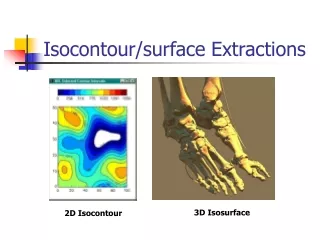
1. Isocontour/surface Extractions 3D Isosurface 2D Isocontour

2. p5 p4 Isocontour (0) Remember bi-linear interpolation p2 p3 To know the value of P, we can first compute p4 and P5 and then linearly interpolate P P =? p1 p0

3. p2 p3 p1 p0 Isocontour (1) Consider a simple case: one cell data set The problem of extracting an isocontour is an inverse of value interpolation. That is: Gieven f(p0)=v0, f(p1)=v1, f(p2)=v2, f(p3)=v3 Find the point(s) P within the cell that have values F(p) = C

4. p2 p3 p1 p0 Isocontour (2) We can solve the problem based on linear interpolation (1) Identify edges that contain points P that have value f(P) = C (2) Calculate the positions of P (3) Connect the points with lines

5. If v1 < C < v2 then the edge contains such a point v1 v2 Isocontouring – Step 1 (1) Identify edges that contain points P that have value f(P) = C

6. Use linear interpolation: P = P1 + (C-v1)/(v2-v1) * (P2 – P1) p1 P p2 v1 v2 C Isocontouring – Step 2 (2) Calculate the position of P

7. Connect the points with line(s) p2 p3 p1 p0 Isocontouring – Step 3 Based on the principle of linear variation, all the points on the line have values equal C

8. p2 p3 So there can be 2 * 2 * 2 * 2 = 16 cases! p1 p0 Isocontour cases How many cases can an isocontour intersect a cell? When comparing the value of Pi with the isovalue C, there can be two cases: Vi > = C or Vi < C

9. (2) One inside(outside), 3 outside(inside) (1) Complete outside(inside) (3) Two inside(outside), two outside(inside) (4) Two contours pass through How many cases again? In fact, there are only 4 unique topological cases

10. p2 p2 p3 p3 p1 p1 p0 p0 - - + outside cell inside cell Inside or Outside? • Just a naming convention • If a value is smaller than the isovalue, we call it “Inside” • If a value is greater than the isovalue, we call it “Outise”

11. Put it all together • Divide-and-conquer algorithm • Look at one cell at a time • Compare the values at 4 vertices with the isovalue C • Linear interpolate along the edges • Connects the interpolated points together

12. 3D Isocontour (Isosurface)

13. Isosurface Extraction • Extend the same divide-and-conquer algorithm to three dimension • 3D cells • Look at one cell at a time • Let’s only focus on voxel

14. _ + + _ _ + + _ _ + + _ _ + + _ Divide-and-Conquer (2 triangles)

15. Now we have 8 vertices So it is: 2 = 256 8 How many unique topological cases? How many cases?

16. _ _ + + _ + + _ _ _ + + _ + _ + Case Reduction (1) Value Symmetry

17. _ _ _ _ _ + _ + _ _ _ _ _ _ + + Case Reduction (2) Rotation Symmetry By inspection, we can reduce 256 14

18. Isosurface Cases Total number of cases: 14

19. Marching Cubes Algorithm A Divide-and-Conquer Algorithm Vi is ‘1’ or ‘0’ (one bit) 1: > C; 0: <C (C= sovalue) Each cell has an index mapped to a value ranged [0,255] Index = v8 v7 v6 v5 v4 v3 v2 v1 v8 v7 v4 v3 v6 v5 v2 v1

20. Marching Cubes (2) Given the index for each cell, a table lookup is performed to identify the edges that has intersections with the isosurface Index intersection edges 0 e1, e3, e5 e7 … 1 e11 e8 e12 e6 2 e3 e5 3 e2 e4 e9 e10 e1 14

21. + _ + _ + _ + _ Marching Cubes (3) • Perform linear interpolations • at the edges to calculate the • intersection points • Connect the points

22. Why is it called marching cubes? • Linear search through cells • Row by row, layer by layer • Reuse the interpolated points • for adjacent cells