Download
1 / 37
370 likes | 565 Views
Enhance your understanding of pre-calculus concepts with Dr. Eddie Ortiz Roman's comprehensive 12th-grade course. Covers graphs, functions, polynomials, exponential functions, trigonometry, vectors, and more.

E N D
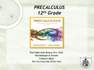
PRECALCULUS12th Grade Prof. Eddie Ortiz Roman, M.S , Ph.D. Microbiologist & Scientist Lehman College The City University of New York
Course Goals • Chapter I. Graphs • 1.1 : The Distance and Mid Point Formulas; Graphing Utilities; • Introduction to Graphing Equations. • 1.2: Intercepts Symmetry; Graphing Key Equations. • 1.3: Solving Equations Using a Graphing Utilities. • 1.4: Lines • 1.5: Circles • Chapter II. Functions and their Graphs. • 2.1 Functions • 2.2 The Graph of a Function. • 2.3 Properties of Functions. • 2.4 Library of Functions; Piecewise-defined functions.
Course Goals • 2.5 Graphing Techniques: Transformations • 2.6: Mathematical Models: Building Functions • Chapter III. Linear & Quadratic Functions. • 3.1: Properties of Linear Functions & Linear Models. • 3.2 Building Linear Models from Data. • 3.3: Quadratic Functions and their Properties. • 3.4: Build Quadratic Models from Verbal Descriptions & rom Data. • Inequalities Involving Quadratic Functions. • Chapter IV. Polynomial & Rational Functions. • 4.1 Polynomial Function & Models. • 4.2The Real Zeros of a Polynomial Function.
Course Goals • 4.3 Complex Zeros; Fundamental • 4.4 Properties of Rational Functions. • 4.5 The Graph of Rational Functions. • 4.6 Polynomial and Rational Inequalities. • Chapter V Exponential & Logarithmic Functions. • 5.1 Composite Functions. • 5.2 One to One Functions; Inverse Functions. • 5.3 Exponential Functions. • 5.4 Logarithmic Functions. • 5.5 Properties of Logarithms • 5.6 Logarithmic and Exponential Functions.
Course Goals • 5.7 Financial Models. • 5.8 Exponential Growth and Decay Models: Newton's Law; • Logistics Growth & Decay Models. • 5.9 Building Exponential, Logarithmic & Logistic Models from Data. • Chapter VI Trigonometric Functions. • Trigonometric Functions • 6.1 Angles and their Measure • 6.2 Trigonometric Functions: Unit Circle Approach • 6.3 Properties of the Trigonometric Functions. • 6.4 Graph of the Sine and Cosine Functions. • 6.5 Graph of the Tangent, Cotangent, Cosecant & Secant Functions. • 6.6 Phase Shift; Sinusoidal Curve Fitting.
Course Goals • Chapter VII Analytic Trigonometry • 7.1 The Inverse Sine, Cosine & Tangent Functions. • 7.2 The Inverse Trigonometric Functions ( Continued ) • 7.3 Trigonometric Equations. • 7.4 Trigonometric Identities. • 7.5 Sum of Difference Formulas. • 7.6 Double – angle and Half angle formulas. • 7.7 Product – to – Sum & Sum – to – Product Formulas. • Chapter VIII: Applications of Trigonometric Functions. • 8.1 Right Triangle Trigonometry Applications. • 8.2 The Law of Sines.
Course Goals • 8.3 The Law of Cosines. • 8.4 Area of a Triangle. • 8.5 Simple Harmonic Function; Damped Motion; Combining Waves. • Chapter XIX Polar Coordinates ; Vectors • 9.1 Polar Coordinates • 9.2 Polar Equations & Graph • 9.3 The Complex Plane; De Moivré's Theorem. • 9.4 Vectors • 9.5 The Dot Product • 9.6 Vectors in Space • 9.7 The Cross Product
Course Goals • Chapter X Analytic Geometry • 10.1 Conics • 10.2 The Parabola • 10.3 The Ellipse • 10.4 The Hyperbola • 10.5 Rotation of Axes; General Form of a Conic • 10.6 Polar Equations of Conics • 10.7 Plane Curves and Parametric Equations. • Chapter XI. Systems of Equations and Inequalities • 11.1 Systems of Linear Equations: Substitutions & Eliminations • 11.2 Systems of Linear Equations: Matrices
Course Goals • 11.3 Systems of Linear Equations; Determinants • 11.4 Matrix Algebra • 11.5 Partial Fraction Decomposition. • 11.6 Systems of Non Linear Equations • 11.7 Systems of Inequalities • 11.8 Linear programming • Chapter XII. Sequences; Induction; The Binomial Theorem. • 12.1 Sequences • 12.2 Arithmetic Sequences • 12.3 Geometric Sequences.; Geometric Series
Course Goals • 12.4 Mathematical Induction. • 12.5 The binomial Theorem • Chapter XIII. Counting & Probability • 13.1 Counting • 13.2 Permutations & Combinations • 13.3 Probability • Chapter XIV A Preview of Calculus; The Limit; Derivative and Integrals of Function. • 14.1 Finding Limits using Tables and Graph. • 14.2 Algebra Techniques for Finding Limits • 14.3 One-side Limits ; Continuous Functions
Course Goals • 14.4 The Tangent Problem; The Derivative • 14.5 The Area Problem; The Integral • A. Review • A.1 Algebra Essentials. • A.2 Geometry Essentials. • A.3 Polynomials. • A.4 Synthetic Division • A.5 Rational Expressions • A.6 Solving Equations. • A.7 Complex Numbers; Quadratic Equations in the Numbers • Complex Systems
Course Head • Dr. Eddie Ortiz Roman, Ph.D( dreortizmd1961@yahoo.com )(eortizasr@gmail.com)Academia Santa Rosa6:00 am – 2:40 pm
What is Pre- Calculus? • Pre-Calculus is a math course that helps students learn the skills and concepts needed to understand calculus. Calculus is the study of change in mathematics. • Pre-Calculus isn't a separate area of study from algebra, trigonometry, coordinate geometry or calculus; rather, it combines elements of all three areas of study.
History of Pre-Calculus • Sir Isaac Newton is credited with inventing calculus (and therefore Pre-Calculus), but there is a lot of debate about that. Some say that Gottfried Wilhelm Leibniz was the true inventor of calculus because he published the first paper on differential calculus in 1684. However, others claim that Sir Isaac Newton gave Gottfried Wilhelm Leibniz the ideas first in a private conversation. The argument of who invented calculus divided the mathematical world, leading even to a broader debate about all of Newton's theories, including his theory of gravitation. In the 400 years following Leibniz's first publication, calculus (and Pre-calculus) has developed from a concept with a small school of adherents in the mathematical world to a course studied in mainstream primary education.
Pre- Calculus problems • Pre-Calculus covers a variety of mathematical problems, from algebra to trigonometry and beyond. However, Pre-Calculus is usually associated with the use of functions, or the graphing of algebraic equations. Pre-Calculus also includes the study of trigonometric equations, linear inequalities, logarithms and exponentials. Usually the student arrives in a Pre-Calculus class already having learned trigonometry, linear inequalities and some basic functions. The goal of Pre-Calculus is to connect those concepts with the higher-order mathematical problems that are part of calculus.
Uses of Pre-Calculus & Calculus • Pre-Calculus is widely used in the engineering and scientific fields, as well as in business. Pre-Calculus is useful in the study of economics, particularly in the use of economic models such as the input-output model that analyzes supply and demand trends. • Pre-calculus is also useful in engineering, especially in studying the resiliency and reactions of building materials and structures under various weather conditions, as well as in physics to explain and graph rates of change. Chemistry also uses Pre-Calculus to quantify chemical reactions
Rectangular Coordinate System Objective: 1) Plot Points using the Rectangular Coordinate System. 2) Calculate the distance between any two points. 3) Determine the midpoint between any two pints. 4) Define – What is a Coordinate Plane and its Quadrants? 5) What is an Axis? 6) Identify the value of its Quadrants. 7) What is an Origin? 8) Identify each ordered pair.
Chapter I. • Rectangular Coordinate System • The rectangular coordinate system consist of two real number lines that intersect at a right angle. The horizontal number line is called the x-axis, and the vertical line is called the y-axis. • These two number lines define a flat surface called a plane, and each point on this plane is associated with an ordered pair of real numbers ( x , y ). The first number is called the x – coordinate, and the second number is called the y-coordinate. The intersection of these two axes is known as the origin, which corresponds to the points ( 0 , 0 )
v vertical Horizontal
An ordered pair ( x , y ) represents the position of the point relative to the origin. The x – coordinate represents the position to the right of the origin if it is positive and to the left of the origin if it is negative. • The y-coordinate represents position above the origin if its positive and below the origin if its negative. Using this system, every position ( point ) in the plane is uniquely identified.
For example, the pair ( 2 , 3 ) denotes the position relative to the origin as shown.
The System is often called “ The Cartesian Coordinate System” named after a French mathematician called • Rene Descartes ( 1596 1650 ) • René Descartes, (born March 31, 1596, La Haye, Touraine, France—died February 11, 1650, Stockholm, Sweden), French mathematician, scientist, and philosopher. Because he was one of the first to abandon scholastic Aristotelianism, because he formulated the first modern version of mind-body dualism, from which stems the mind-body problem, and because he promoted the development of a new science grounded in observation and experiment, he has been called the father of modern philosophy. Applying an original system of methodical doubt, he dismissed apparent knowledge derived from authority, the senses, and reason and erected new epistemic foundations on the basis of the intuition that, when he is thinking, he exists; this he expressed in the dictum “I think, therefore I am” (best known in its Latin formulation, “Cogito, ergo sum,” though originally written in French, “Je pense, donc je suis”). He developed a metaphysical dualism that distinguishes radically between mind, the essence of which is thinking, and matter, the essence of which is extension in three dimensions. Descartes’s metaphysics is rationalist, based on the postulation of innate ideas of mind, matter, and God, but his physics and physiology, based on sensory experience, are mechanistic and empiricist.
The x and y axes breaks the plane into four regions called “ Quadrants” named using Roman Numerals I, II, III, IV as pictured as pictured, In Quadrant I both coordinates are positive. In Quadrant II, the x coordinate is negative and the y coordinate is positive. In Quadrant III, both coordinates are negative and in Quadrant IV the x coordinate is positive and the y coordinate is negative.
Distance Formula Frequently you need to calculate the distance between two points in a plane. To do this, form a right triangle using the two points as vertices of the triangle and then apply the Pythagorean Theorem states that is given any right angle with legs measuring a + b units, then the square of the measure of the hypotenuse “ c ” is equal to the sum of the square of the legs. Formula: a2 + b2 = c2 “ In other words: The hypotenuse of any right triangle is equal to the square root of the sum of the square of its legs.
What is a mid point of a line segment ? A midpoint of a line segment is a point that is halfway between the end points of the line segments. We can use this formula: M = ( xA+xB2 , yA+yB2 ) Example: What is the midpoint here? Midpoint of Line Use the formula: M = ( xA+x , yA+yB ) 2 2 M = ( (−3)+8 , 5+(−1) ) 2 2 M = ( 5/2, 4/2 ) M = ( 2.5, 2 )
Chapter I The Distance & Midpoint FormulasGraphing Utilities: Introduction to Graphing Equations Objective. • Use the Distance Formula. • Use the Midpoint Formula • Graph Equations by Plotting Points. • Graph Equations using a Graphing Utility. • Use a graphing utility to create tables. • Find Intercepts from a Graph. • Use a Graphing Utility to approximate intercepts.
Finding the Distance been 2 points. Chapter 1.1 Find the distance “d” between the points ( 1,3) and ( 5,6). Solution First plot the points (1,3) and (5,6) and connect them with a straight line. ( 5,6 ) ( 1,3 ) ( 5,3 ) d2 = 42 + 32 = 16 + 9 = 25 The distance formula provides a straightforward method for computing the distance between two points.
Theorem: Distance Formula The distance formula between two points P1 = ( x1 , y1 ) and P2 = ( x2 , y2 ) denoted by d ( P1 , P2 ) is d ( P1 , P2 ) = ( x2 – x1 )2 + ( y2 – y1 )2 Example: P2 = ( X2 , Y2 ) d ( P1 , P2 ) Y2 – Y1 P1 = ( X1 . Y1 ) X2 – X1
Proof of the Distance Formula Pg #4 Let ( x1 , y1 ) denote the coordinates of point P1 , and let ( x2,y2 ) denotes the coordinates of P2, assume that the line joining P1 and P2 is neither horizontal nor vertical. The coordinates of P3 are ( x2, y1 ). The horizontal distance from P1 to P3vis the absolute value of the difference of the x-coordinates x2 – x1 The vertical distance from P3 to P2 is the absolute value of the difference of the y-coordinates. The distance d ( P1 , P2 ) is the length of the hypotenuse of the right triangle, so by the Pythagorean Theorem It follows that: see next page ( example )
( d ( P1 , P2 ) 2 = x2 – x12 + y2 – y12 = ( x2 – x1 )2 + ( y2 – y1 ) 2 d ( P1, P2 = ( x2 – x1)2 + ( y2 – y1 )2 In words: To compute the distance between two points , find the distance of the x-coordinates, square it, and add this to the square of the difference of the y-coordinates. The square root of of this sum is the distance. Example:
Example y y y2 -P2= ( x2 , y2 ) y2 P2= ( x2 , y2 ) d ( P1, P2 ) y2 – y1 y1 y1 P1 = ( x1 , y1 ) P3 = ( x2 , y1) P1 = ( X1,Y1 ) ( X2 – X1 )P3 = ( x2 , y1 ) x x x1 x2 x1 x2
Grading Scale • Could be adjusted for equity (“on the curve”)—up, but not down • Pluses and minuses will also be determined in final analysis
Text • PreCalculus • Enhance with Graphing Utilities • Seventh Edition • Author: Sullivan & Sullivan
For those who have taken AP Calculus BC • Math 1a and 1b together cover the Calculus BC syllabus • Math 1b does more than what’s on the BC, with different emphasis • You will still find lots to learn in Math 1b
For those who have taken AP Calculus AB • Some of your classmates will have seen some of this material before • We are committed to supporting all qualified students
Conclusion • I hope you enjoy the conference • Web site reminder: ( dreortizmd1961@yahoo.com ) • ( eortizasr@gmail.com) • Academia Santa Rosa de Lima