Download
1 / 19
190 likes | 358 Views
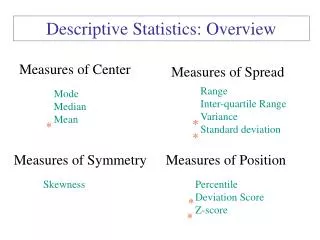
Descriptive Statistics-III (Measures of Central Tendency). QSCI 381 – Lecture 5 (Larson and Farber, Sects 2.3 and 2.5). Introduction. is a value that represents the typical, or central, entry in a data set.

E N D
Descriptive Statistics-III(Measures of Central Tendency) QSCI 381 – Lecture 5 (Larson and Farber, Sects 2.3 and 2.5)
Introduction • is a value that represents the typical, or central, entry in a data set. • There are three commonly used measures of central tendency: • The Mean • The Median • The Mode. A Measure of Central Tendency
The Mean-I • The sample mean: • The population mean:
The Mean-II • Consider the data set consisting of a sample of the diameters of 6 trees in a stand: 29cm, 31cm, 43cm, 31cm, 12cm, 33cm • Calculate the mean:
The Mean-III • Why we like the mean • Unique. • Based on every data point in the data set. • Well suited to statistical treatment. • Why we dislike the mean • Can be sensitive to “outlying” observations.
The Median • Sort the data and average the central values. • Six values: • Five values: 32 31
The Mode • Find the frequency of each data entry and identify the data entry with the greatest frequency. • Unlike the median and mean, the mode is not always uniquely defined. If a data set has two modes, it is referred to as being bimodal.
Which Measure is Best? • There is no clear answer to this question. • The mean can be influenced by outliers while the mode may not be particularly “typical”. • Statistical inference based on the median and the mode is somewhat difficult. Median Mode Mean Outlier?
Computing the Mean of a Group of Data Points • Suppose the data are in the form of frequencies, i.e., for each i, we have xi and fi, where fi is number of data entries for which x equals xi, then: In Excel use: “sumproduct(a1:a10,b1:b10)/sum(b1:b10)” where the xi’s are stored in column A and the fi’s are stored in column B.
Shapes of Distributions-I • A frequency distribution is when a vertical line can be drawn through the middle of a graph of the distribution and the resulting halves are mirror images. Symmetric Mean, Median, Mode
Shapes of Distributions-II • A frequency distribution is (or rectangular) when the number of entries in each class is equal (a uniform distribution is symmetric). Uniform Mean, Median, Mode
Shapes of Distributions-III • A frequency distribution is (or positively skewed) if its tail extends to the right (mode < median < mean). Skewed right Mode Median Tail Mean
Shapes of Distributions-IV • A frequency distribution is (or negatively skewed) if its tail extends to the left (mode > median > mean). Skewed left
Fractiles Range • The is the difference between the maximum and minimum data entries. • The : Q1, Q2, and Q3, divide a (ordered) data set into four equal parts. • The : P1, P2, ….P99 divide a (ordered) data set into 100 equal parts. • Collectively, Quartiles, Percentiles (and Deciles) are referred to as Fractiles. Quartiles Percentiles
More on Quartiles • The quartiles divide a data set at the 25th percentile, the 50th percentile, and the 75th percentile. • The 50th percentile is the median. • The difference between the 75th and 25th percentiles is referred to as the . Interquartile range
More on Percentiles 80% 15.2m Interpretation: 80% of the bowheads caught are smaller than 15.2m
Box and Whisker Plots-I • The information on the range and the quartiles can be represented using a box and whisker plot.
Box and Whisker Plots-II • Find the five number summary of the data (range, Q1,Q2,Q3). • Construct a horizontal line that spans the data. • Plot the five numbers above the horizontal scale. • Draw a box above the horizontal scale from Q1 to Q3 and draw a vertical line in the box at Q2. Q1 Q2 Median Q3 Maximum Minimum whisker 5 10 15 Length (m)