Download
1 / 35
380 likes | 491 Views
Inverse Problems in Geophysics. What is an inverse problem? - Illustrative Example - Exact inverse problems - Nonlinear inverse problems Examples in Geophysics - Traveltime inverse problems - Seismic Tomography - Location of Earthquakes - Global Electromagnetics

E N D
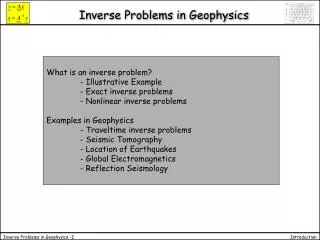
Inverse Problems in Geophysics What is an inverse problem? - Illustrative Example - Exact inverse problems - Nonlinear inverse problems Examples in Geophysics - Traveltime inverse problems - Seismic Tomography - Location of Earthquakes - Global Electromagnetics - Reflection Seismology
What is an inverse problem? Forward Problem Model m Data d Inverse Problem
Treasure Hunt X X X X Gravimeter ?
Treasure Hunt – Forward Problem We have observed some values: 10, 23, 35, 45, 56 gals How can we relate the observed gravity values to the subsurface properties? We know how to do the forward problem: X X X X X Gravimeter ? This equation relates the (observed) gravitational potential to the subsurface density. -> given a density model we can predict the gravity field at the surface!
Treasure Hunt – Trial and Error What else do we know? Density sand: 2,2 g/cm3 Density gold: 19,3 g/cm3 Do we know these values exactly? How can we find out whether and if so where is the box with gold? X X X X X Gravimeter ? One approach: Use the forward solution to calculate many models for a rectangular box situated somewhere in the ground and compare the theoretical (synthetic) data to the observations. ->Trial and error method
Treasure Hunt – Model Space But ... ... we have to define plausible models for the beach. We have to somehow describe the model geometrically. -> Let us - divide the subsurface into rectangles with variable density - Let us assume a flat surface X X X X X Gravimeter ? x x x x x surface sand gold
Treasure Hunt – Non-uniqueness • Could we go through all possible models • and compare the synthetic data with the • observations? • at every rectangle two possibilities • (sand or gold) • 250 ~ 1015 possible models • Too many models! X X X X X Gravimeter • We have 1015 possible models but only 5 observations! • It is likely that two or more models will fit the data (possibly perfectly well) • > Nonuniqueness of the problem!
Treasure Hunt – A priori information • Is there anything we know about the • treasure? • How large is the box? • Is it still intact? • Has it possibly disintegrated? • What was the shape of the box? • Has someone already found it? • This is independent information that we may have which is as important and • relevant as the observed data. This is colled a priori (or prior) information. • It will allow us to define plausible, possible, and unlikely models: X X X X X Gravimeter plausible possible unlikely
Treasure Hunt – Uncertainties (Errors) • Do we have errors in the data? • Did the instruments work correctly? • Do we have to correct for anything? • (e.g. topography, tides, ...) • Are we using the right theory? • Do we have to use 3-D models? • Do we need to include the topography? • Are there other materials in the ground apart from gold and sand? • Are there adjacent masses which could influence the observations? • How (on Earth) can we quantify these problems? X X X X X Gravimeter
X X X X X Gravimeter Treasure Hunt - Example Models with less than 2% error.
X X X X X Gravimeter Treasure Hunt - Example Models with less than 1% error.
X X X X X Gravimeter Inverse Problems - Summary Inverse problems – inference about physical systems from data • Data usually contain errors (data uncertainties) • Physical theories are continuous • infinitely many models will fit the data (non-uniqueness) • Our physical theory may be inaccurate (theoretical uncertainties) • Our forward problem may be highly nonlinear • We always have a finite amount of data • The fundamental questions are: • How accurate are our data? • How well can we solve the forward problem? • What independent information do we have on the model space (a priori information)?
Corrected scheme for the real world Forward Problem True Model m Data d Appraisal Problem Inverse Problem Estimated Model
Exact Inverse Problems • Examples for exact inverse problems: • Mass density of a string, when all eigenfrequencies are known • Construction of spherically symmetric quantum mechanical potentials • (no local minima) • 3.Abel problem: find the shape of a hill from the time it takes for a ball • to go up and down a hill for a given initial velocity. • 4. Seismic velocity determination of layered media given ray traveltime • information (no low-velocity layers).
Abel’s Problem (1826) z P(x,z) dz’ ds x Find the shape of the hill ! For a given initial velocity and measured time of the ball to come back to the origin.
z P(x,z) dz’ ds At any point: x At z-z’: After integration: The Problem
z P(x,z) dz’ ds x The solution of the Inverse Problem After change of variable and integration, and...
Wiechert-Herglotz Inversion The solution to the inverse problem can be obtained after some manipulation of the integral : forward problem inverse problem The integral of the inverse problem contains only terms which can be obtained from observed T(D) plots. The quantity 1=p1=(dT/dD)1 is the slope of T(D) at distance D1.The integral is numerically evaluated with discrete values of p(D) for all D from 0 to D1. We obtain a value for r1 and the corresponding velocity at depth r1 is obtained through 1=r1/v1.
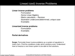
Linear(ized) Inverse Problems Let us try and formulate the inverse problem mathematically: Our goal is to determine the parameters of a (discrete) model mi, i=1,...,m from a set of observed data djj=1,...,n. Model and data are functionally related (physical theory) such that This is the nonlinear formulation. Note that mi need not be model parameters at particular points in space but they could also be expansion coefficients of orthogonal functions (e.g. Fourier coefficients, Chebyshev coefficients etc.).
Linear(ized) Inverse Problems If the functions Ai(mj) between model and data are linear we obtain or in matrix form. If the functions Ai(mj) between model and data are mildly non-linear we can consider the behavior of the system around some known (e.g. initial) model mj0:
Linear(ized) Inverse Problems We will now make the following definitions: Then we can write a linear(ized) problem for the nonlinear forward problem around some (e.g. initial) model m0 neglecting higher order terms:
Linear(ized) Inverse Problems • Interpretation of this result: • m0 may be an initial guess for our physical model • We may calculate (e.g. in a nonlinear way) the synthetic data d=f(m0). • We can now calculate the data misfit, Dd=d-d0, where d0 are the observed data. • Using some formal inverse operator A-1 we can calculate the corresponding model perturbationDm. This is also called the gradient of the misfit function. • We can now calculate a new model m=m0+ Dm which will – by definition – is a better fit to the data. We can start the procedure again in an iterative way.
Nonlinear Inverse Problems Assume we have a wildly nonlinear functional relationship between model and data The only option we have here is to try and go – in a sensible way – through the whole model space and calculate the misfit function and find the model(s) which have the minimal misfit.
Model Search • The way how to explore a model space is a science itself! • Some key methods are: • Monte Carlo Method: Search in a random way through the model space and collect models with good fit. • Simulated Annealing. In analogy to a heat bath, or the generation of crystal one optimizes the quality (improves the misfit) of an ensemble of models. Decreasing the temperature would be equivalent to reducing the misfit (energy). • Genetic Algorithms. A pool of models recombines and combines information, every generation only the fittest survive and give on the successful properties. • Evolutionary Programming. A formal generalization of the ideas of genetic algorithms.
Inversion: the probabilistic approach The misfit function can also be interpreted as a likelihood function: describing a probability density function (pdf) defined over the whole model space (assuming exact data and theory). This pdf is also called the a posteriori probability. In the probabilistic sense the a posteriori pdf is THE solution to the inverse problem.
Examples: Seismic Tomography Data vector d: Traveltimes of phases observed at stations of the world wide seismograph network Model m: 3-D seismic velocity model in the Earth’s mantle. Discretization using splines, spherical harmonics, Chebyshev polynomials or simply blocks. Sometimes 10000s of travel times and a large number of model blocks: underdetermined system
Examples: Earthquake location Seismometers Data vector d: Traveltimes observed at various (at least 3) stations above the earthquake Model m: 3 coordinates of the earthquake location (x,y,z). Usually much more data than unknowns: overdetermined system
Examples: Global Electromagnetism Data vector d: Amplitude and Phase of magnetic field as a function of frequency Model m: conductivity in the Earth’s mantle Usually much more unknowns than data: underdetermined system
Examples: Reflection Seismology Air gun Data vector d: ns seismograms with nt samples -> vector length ns*nt Model m: the seismic velocities of the subsurface, impedances, Poisson’s ratio, density, reflection coefficients, etc. receivers
Inversion: Summary • We need to develop formal ways of • calculating an inverse operator for • d=Am -> m=A-1d • (linear or linearized problems) • describing errors in the data and theory (linear and nonlinear problems) • searching a huge model space for good models (nonlinear inverse problems) • describing the quality of good models with respect to the real world (appraisal).