Download
1 / 22
230 likes | 509 Views
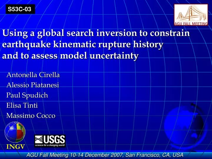
INGV. S53C-03. Using a global search inversion to constrain earthquake kinematic rupture history and to assess model uncertainty. Antonella Cirella Alessio Piatanesi Paul Spudich Elisa Tinti Massimo Cocco. AGU Fall Meeting 10-14 December 2007, San Francisco, CA, USA . Goals:.

E N D
INGV S53C-03 Using a global search inversion to constrain earthquake kinematic rupture history and to assess model uncertainty Antonella Cirella Alessio Piatanesi Paul Spudich Elisa Tinti Massimo Cocco AGU Fall Meeting 10-14 December 2007, San Francisco, CA, USA
Goals: 1. Global search kinematic inversion technique of seismological & geodetic data; 2. Assessment of kinematic model uncertainty; 3. Applications: 2007 Niigata & 2000 Tottori Earthquakes; 4. Dynamic consistency of kinematic models; AGU Fall Meeting 10-14 December 2007, San Francisco, CA, USA
2) finite fault is divided into sub-faults; • Inverted Parameters: • Peak Slip Velocity; • Rise Time; • Rupture Velocity; • Rake. Kinematic Inversion:Data & Fault Parameterization 1) joint inversion of strong motion and GPS data; 3) kinematic parameters are allowed to vary within a sub-fault; 4) several analytical slip velocity source time functions (STFs) are implemented. AGU Fall Meeting 10-14 December 2007, San Francisco, CA, USA
START random model m0 Loop over model values M loop over parameters N (Vr,rise time,…) Forward Modeling: DWFE Method - Compsyn (complete response 1D vertically varying Earth Structure) To quantify the misfit… Strong motionL1+L2 norm GPS L2 norm = + END : Minimum Value of the Cost Function Multiple Restart Kinematic Inversion:Stage I: Building Model Ensemble–HB Simulated Annealing AGU Fall Meeting 10-14 December 2007, San Francisco, CA, USA
Kinematic Inversion:Appraisal of the Ensemble Model Ensemble Inference Rather then simply looking at the best model, we extract the most stable features of the rupture process that are consistent with the data and give us an estimate of the variability of each model parameter. “Limiting the analysis to the features present in only the best fitting model is often insufficient because of non-uniqueness in the problem and noise in the data “ (e.g. Mosegaard & Sambridge, 2002). AGU Fall Meeting 10-14 December 2007, San Francisco, CA, USA
Kinematic Inversion:Stage II: Appraisal of the Ensemble Output of kinematic inversion: Ω Rupture Models m & Cost Function C(m) Cost Function Model Ensemble Ω = iterations • Standard Deviation: • Best Model: • Average Model: AGU Fall Meeting 10-14 December 2007, San Francisco, CA, USA
13 stations (surface or borehole strong motion records); • 15 GPS stations ; • frequency-band: (0.02÷0.5)Hz; • 60 sec (body & surface waves); • South-East Dipping Fault; http://www.eqh.dpri.kyoto-.ac.jp/~mori/niigata/reloc.html Kinematic Inversion: 2007 Niigata-ken Chuetsu-oki Earthquake, Mw=6.6 July 16-th 2007 • W=31.5km; L=38.5km; =3.5km; • all kinematic parameters are inverted simultaneously.
Best Model: C(m)=0.3 vs Average Model: C(m)=0.4 SW NE • The best fitting model might contain an extreme configuration of model parameters; • The ensemble-averaged model better represents the stable features of the rupture history.
Strong Motion Comparison between synthetics (red) and observed (blue) waveforms. GPS Comparison between synthetics (white) and observed (red) coseismic horizontal displacement.
Kinematic Inversion:Source Time Function Cosine Regularized Yoffe Tacc=0.2sec Regularized Yoffe Tacc=0.4sec Tacc The slip velocity history on each point on the fault is determined by the shape of the a priori assumed source time function (single window approach). Box-car GOAL: to understand the importance of adopting source time functions, compatible with EQ dynamics to image rupture history on a finite-fault. AGU Fall Meeting 10-14 December 2007, San Francisco, CA, USA
18 stations (surface & borehole strong motion records); • 14 GPS stations ; • frequency-band: (0.05÷1.00)Hz; Kinematic Inversion: 2000 Western Tottori Earthquake, Mw=6.6 October 6-th 2000 • W=20 km; L=40 km; =4 km • all kinematic parameters are inverted simultaneously; • 4 different STFs are adopted. AGU Fall Meeting 10-14 December 2007, San Francisco, CA, USA
SLIP SLIP SLIP SLIP PSV RISE PSV RISE PSV RISE RISE PSV Results – Kinematic Parameters Box Cos Y0.2 Y0.4 AGU Fall Meeting 10-14 December 2007, San Francisco, CA, USA
DYNAMIC MODELING • Traction Evolution; • Dynamic Stress Drop; • Dc Kinematic Inversion Dynamic Modeling KINEMATIC MODELS • Slip; • Rupture Time; • Rise Time; • Rake; • Source Time Function AGU Fall Meeting 10-14 December 2007, San Francisco, CA, USA
Dynamic Parameters1: Dynamic Stress Drop • Dynamic Stress Drop (τo - τd) distribution on the fault; the box-car yields the highest values; the two Yoffe give very similar stress drop distributions both in shape and in amplitude; the cosine produces a rupture with lowest stress drop. AGU Fall Meeting 10-14 December 2007, San Francisco, CA, USA
Traction vs Slip Curves; Dc=Dtot Dc Dtot Dt (subfault with maximum slip); Dynamic Parameters2: Traction Time Histories • Details of Traction, Slip & Slip Velocity Time Histories; AGU Fall Meeting 10-14 December 2007, San Francisco, CA, USA
Conclusions • The proposed methodology allows us to jointly invert seismological & geodetic data in order to image the kinematic rupture history for extended sources; • It provides a robust estimate of the stable features of rupture history constraining the variability of model parameters; • By using different STFs we emphasize the importance of adopting dynamically consistent functions in kinematic inversions, since kinematic rupture models are often used to constrain dynamic traction evolution; • Our preliminary inverted source model for the 2007 Niigata, Japan, earthquake shows several interesting features (non-uniform rupture velocity, heterogeneous slip distribution, ….) which require further analyses AGU Fall Meeting 10-14 December 2007, San Francisco, CA, USA
Kinematic Inversion:Cost Function Strong motionL1+L2 norm Spudich & Miller, 1990 GPS L2 norm Hudnut, 1996 AGU Fall Meeting 10-14 December 2007, San Francisco, CA, USA
Relocation of Aftershocks of the 2007 Niigata-ken Chuetsu Oki Earthquake Early Aftershocks (10:13 to 15:36) These plots show the aftershock distributions before the time of the largest aftershock (M5.8) at 15:37. The mainshock location (star) was not determined with this procedure. There appears to be a fairly clear eastward dipping trend from the time of the mainshock. References Evans, J., D. Eberhart-Phillips, C. H. Thurber, User's manual for SIMULPS12 for imaging vp and vp/vs: A derivative of the "Thurber" tomographic inversion SIMUL3 for local earthquakes, USGS Open-File Report 94-431, 1994. Shibutani, T., H. Katao and Group for the dense aftershock observations of the 2000 Western Tottori Earthquake, High resolution 3-D velocity structure in the source region of the 2000Western Tottori Earthquake in southwestern Honshu, Japan using very dense aftershock observations, Earth Planets Space, 57, 825-838, 2005 Waldhauser, F., hypoDD: A program to compute double-difference hypocenter locations, USGS Open-File Report, 01-113, 2001. Zhang, H. and C.H. Thurber, Double-difference tomography: the method and its application to the Hayward fault, California, Bull Seismol. Soc. Am., 93, 1875-1889, 2003.
Strong Motion Best Model Comparison between synthetics (red) and observed (blue) waveforms. GPS Comparison between synthetics (white) and observed (red) coseismic horizontal displacement.
Strong Motion STF: Yoffe 0.400; Average model. Comparison between synthetics (red) and observed (blue) waveforms. GPS Comparison between synthetics (red) and observed (blue) coseismic horizontal displacement. 10 cm AGU Fall Meeting 10-14 December 2007, San Francisco, CA, USA