Download
1 / 43
430 likes | 554 Views
Spectra and Temporal Variability of Galactic Black-hole X-ray Sources in the Hard State. Nick Kylafis University of Crete This is part of the PhD Thesis of Dimitrios Giannios (MPA) (collaboration with P. Reig and D. Psaltis) Ann Arbor, December 2005.

E N D
Spectra and Temporal Variability of Galactic Black-hole X-ray Sources in the Hard State Nick Kylafis University of Crete This is part of the PhD Thesis of Dimitrios Giannios (MPA) (collaboration with P. Reig and D. Psaltis) Ann Arbor, December 2005
X-ray spectra from sources containing a stellar-mass black hole. • Black-hole X-ray sources appear in two states: • In one state (called soft) the X-ray spectrum is dominated by “soft” X rays (1 – 10 keV) and it is close to a blackbody of temperature kΤ~2 keV. It is generally accepted that these soft X rays come from the accretion disk.
X-ray spectra from sources containing a stellar-mass black hole. • In the other state (called hard) the X-ray spectrum is dominated by “hard” X rays (~1 – 300 keV) and it is a power law of the form
X-ray spectra from sources containing a black hole. • In the other state (called hard) the X-ray spectrum is dominated by “hard” X rays (~1 – 300 keV) and it is a power law of the form • There is also a small blackbody component from the accretion disk with kT ~ 0.2 keV.
X-ray spectra from sources containing a black hole. • In the other state (called hard) the X-ray spectrum is dominated by “hard” X rays (~1 – 300 keV) and it is a power law of the form • There is also a small blackbody component from the accretion disk with kT ~ 0.2 keV. • In this state, a radio jet is always seen.
X-ray spectra from sources containing a black hole. • In the other (called hard) the X-ray spectrum is dominated by “hard” X rays (~1 – 300) keV) and it is a power law of the form • There is also a small blackbody component from the accretion disk with kT ~ 0.2 keV. • In this state, a radio jet is always seen. • It looks as if the inner part of the disk has given rise to the jet.
Schematic picture • Accretion disk with jet.
E 0 How can one produce a spectrum of the form ? • Let’s consider low-energy photons , e.g. from the accretion disk.
E 0 • Let be the mean fractional increase of the photon energy per scattering. Then How can one produce a spectrum of the form ? • Let’s consider low-energy photons , e.g. from the accretion disk.
How can one produce a spectrum of the form ? • If is the probability for a photon to be scattered once, then the intensity of photons scattered times is
How can one produce a spectrum of the form ? • If is the probability for a photon to be scattered once, then the intensity of photons scattered times is • Solving equation (1) for and substituting into (2) we obtain where
Compton up-scattering in the jet. • Our model proposes that low-energy photons (~ 0.1 – 1 keV) from the accretion disk either escape un-scattered or they are scattered by the fast moving electrons in the jet.
Compton up-scattering in the jet. • Our model proposes that low-energy photons (~ 0.1 – 1 keV) from the accretion disk either escape un-scattered or they are scattered by the fast moving electrons in the jet. • It is obvious that electrons in the jet must not only possess but also .
Compton up-scattering in the jet. • Our model proposes that low-energy photons (~ 0.1 – 1 keV) from the accretion disk either escape un-scattered or they are scattered by the fast moving electrons in the jet. • It is obvious that electrons in the jet must not only possess but also . • It is not necessary for the electrons to be thermal, as we will see below. On the contrary.
Typical model X-ray spectrum from Compton up-scattering in a jet.
Comparison with observations. Observed and model spectrum of Cygnus X-1.
Time lags of the hard photons due to scattering. • Do we have any indication that inverse Compton scattering indeed takes place? • It is clear that, if the power-law spectrum is produced by successive Compton scatterings, then the high-energy photons (e.g. 50 – 100 keV), that have scattered many times to get to this energy, must exhibit a time lag w.r.t. the softer photons (e.g. 1 – 10 keV)that have scattered fewer times. • This is indeed observed!!!
Time lags of the hard photons due to scattering. • Let the observed intensities in two energy bands and beand .
Time lags of the hard photons due to scattering. • We take theFourier transforms • Let the observed intensities in two energy bands and beand .
Time lags of the hard photons due to scattering. • We take theFourier transforms • and then the product • Let the observed intensities in two energy bands and beand .
Time lags of the hard photons due to scattering. • A phase difference corresponds to a time lag that is given by
Time lags of the hard photons due to scattering. • A phase difference corresponds to a time lag that is given by • Naively we expect
Time lags of the hard photons due to scattering. • A phase difference corresponds to a time lag that is given by • Naively we expect • What is observed however is that requires a logical explanation.
Time lags and frequency of variability(Fourier frequency). • For simplicity, let’s consider a source of photons of energy that has periodicity only at frequency , i.e., with a period .
Time lags and frequency of variability(Fourier frequency). • For simplicity, let’s consider a source of photons of energy that has periodicity only at frequency , i.e., with a period . • Let be the mean time lag of the photons that scattered many times.
Time lags and frequency of variability(Fourier frequency). • For simplicity, let’s consider a source of photons of energy that has periodicity only at frequency , i.e., with a period . • Let be the mean time lag of the photons that scattered many times. • If, the time lags of the photons DO NOT AFFECT the intrinsic periodicity of the source.
Time lags and frequency of variability(Fourier frequency). • However, if , and because there is a distribution of time lags, the photons FORGET the phase with which they were emitted and thus we do not observe any variability.
Time lags and frequency of variability(Fourier frequency). • However, if , and because there is a distribution of time lags, the photons FORGET the phase with which they were emitted and thus we do not observe any variability. • In other words, large periods of variability are observed, but for or smaller the variability of the source is washed out.
Time lags and frequency of variability(Fourier frequency). • However, if , and because there is a distribution of time lags, the photons FORGET the phase with which they were emitted and thus we do not observe any variability from the source. • In other words, large periods of variability are observed, but for or smaller the variability of the source is washed out. • Equivalently, we can say that Compton scattering acts as a filter that cuts off the high frequencies.
Time lags and frequency of variability(Fourier frequency). • Let’s consider now Compton scatterings in successive regions with larger and larger time lag from region to region. • The larger the time lag, the more Fourier frequencies are washed out.
tlag R3 t3 t3 t2 R2 t2 t1 R1 t1 ν 1/t3 1/t2 1/t1 Schematic picture
Time lags and frequency of variability (Fourier frequency). • We computed as a function of Fourier frequency for a source at the base of the jet.
Time lags and frequency of variability (Fourier frequency). • We computed as a function of Fourier frequency for a source at the base of the jet. • To obtain , the density in the jet must be .
Time lags and frequency of variability (Fourier frequency). • We computed as a function of Fourier frequency for a source at the base of the jet. • To obtain , the density in the jet must be . • For such a density, the mean free path to electron scattering is , and therefore the photons are scattered with the same probability in every decade of distance.
Constraints to our model • There are three additional constraints to our proposed model. • Two of them have to do with the energy dependence of the power density function and the autocorrelation function (discussion at the end if time allows). • The third and most important constraint has to do with the observed radio waves from the jet.
Constraints to our model • Given the density profile in the jet that is required to explain the time lags • and given the velocity distribution of the electrons that is required to explain the X-ray spectrum, • is it possible to explain the observed radio spectrum with NO ADDITION OF OTHER INGREDIENTS to the model?
Constraints to our model. • Fortunately, the answer is YES. • Up to now, for only one source we have simultaneous observation of the energy spectrum from radio to X rays. • The success of the model is surprisingly good.
Comparison of our model with observations. Model and observations forXTE J 1118+480
Conclusions • The proposed model seems to explain all the existing observations. • It is therefore worth more stringent tests. THANKS
Jet model: two more constraints. • The flattening of the power spectrum with increasing photon energy and • the narrowing of the auto-correlation function • can be explained with one additional assumption: • The jet is “hotter” at its center than at its periphery.
Jet model: radio spectrum • With a power-law distribution of electron velocities • not only the radio but the ENTIRE energy spectrum is explained.