Download
1 / 36
360 likes | 511 Views
Topic 10 - Ensemble Methods. Ensemble Models - Motivation. Remember this picture? Always looking for balance between low complexity (‘good on average’ but bad for prediction) and high complexity (‘good for specific cases’ but might overfit)

E N D
Topic 10 - Ensemble Methods Data Mining - Volinsky - 2011 - Columbia University
Ensemble Models - Motivation • Remember this picture? • Always looking for balance between low complexity (‘good on average’ but bad for prediction) and high complexity (‘good for specific cases’ but might overfit) • By combining many different models, ensembles make it easier to hit the ‘sweet spot’ of modelling. • Best for models to draw from diverse, independent opinions • Wisdom Of Crowds Stest(q) Strain(q) Data Mining - Volinsky - 2011 - Columbia University
Ensemble Methods - Motivation • Models are just models. • Usually not true! • The truth is often much more complex than any single model can capture. • Combinations of simple models can be arbitrarily complex. (e.g. spam/robots models, neural nets, splines) • Notion: An average of several measurements is often more accurate and stable than a single measurement Accuracy: how well the model does for estimation and prediction Stability: small changes in inputs have little effect on outputs Data Mining - Volinsky - 2011 - Columbia University
Ensemble Methods – How They Work • The ensemble predicts a target value as an average or a vote of the predictions (of several individual models)... • Each model is fit independently of the others • Final prediction is a combination of the independent predictions of all models • For an continuous target, an ensemble averages predictions • Usually weighted • For a categorical target (classification), an ensemble may average the probabilities of the target values…or may use ‘voting’. • Voting classifies a case into the class that was selected most by individual models Data Mining - Volinsky - 2011 - Columbia University
Ensemble Models – Why they work • Voting example • 5 independent classifiers • 70% accuracy for each • Use voting… • What is the probability that the ensemble model is correct? • Lets simulate it • What about 100 examples? • (not a realistic example, why?) Data Mining - Volinsky - 2011 - Columbia University
Ensemble Schemes • The beauty is that you can average together models of any kind!!! • Don’t need fancy schemes – just average! • But there are fancy schemes: each one has various ways of fitting many models to the same data, and use voting or averaging • Stacking (Wolpert 92): fit many leave-1-out models • Bagging (Breiman 96) build models on many permutations of original data • Boosting (Freund & Shapire 96): iteratively re-model, using re-weighted data based on errors from previous models… • Arcing (Breiman 98), Bumping (Tibshirani 97), Crumpling (Anderson & Elder 98) , Born-Again (Breiman 98): • Bayesian Model Averaging - near to my heart… • We’ll explore BMA, bagging and boosting… Data Mining - Volinsky - 2011 - Columbia University
Ensemble Methods – Bayesian Model Averaging Data Mining - Volinsky - 2011 - Columbia University
Model Averaging • Idea: account for inherent variance of the model selection process • Posterior Variance = Within-Model Variance + Between-Model Variance • Data-driven model selection is risky: “Part of the evidence is spent specify the model” (Leamer, 1978) • Model-based inferences can be over-precise Data Mining - Volinsky - 2011 - Columbia University
Model Averaging • For some quantity of interest D: avg over all Models M, given the data D: To calculate the first term properly, you need to integrate out model parameters q, Where q is the MLE. For the second term, note that ^ Data Mining - Volinsky - 2011 - Columbia University
Bayesian Model Averaging • The approximations on the previous page allow you to calculate many posterior model probabilities quickly, and gives you the weights to use for averaging. • But, how do you know which models to average over? • Example, regression with p parameters • Each subset of p is a ‘model’ • 2p possible models! • Idea: Data Mining - Volinsky - 2011 - Columbia University
Model Averaging • But how to find the best models without fitting all models? • Solution: Leaps and Bounds algorithm can find the best model without fitting all models • Goal: find the single best model for each model size Don’t need to traverse this part of the tree since there is no way it can beat AB Data Mining - Volinsky - 2011 - Columbia University
BMA - Example PMP = Posterior Model Probability Best Models Score on holdout data: BMA wins Data Mining - Volinsky - 2011 - Columbia University
Ensemble Methods - Boosting Data Mining - Volinsky - 2011 - Columbia University
Boosting… • Different approach to model ensembles – mostly for classification • Observed: when model predictions are not highly correlated, combining does well • Big idea: can we fit models specifically to the “difficult” parts of the data? Data Mining - Volinsky - 2011 - Columbia University
Boosting— Algorithm From HTF p. 339 Data Mining - Volinsky - 2011 - Columbia University
Example • Courtesy M. Littman Data Mining - Volinsky - 2011 - Columbia University
Example • Courtesy M. Littman Data Mining - Volinsky - 2011 - Columbia University
Example • Courtesy M. Littman Data Mining - Volinsky - 2011 - Columbia University
Boosting - Advantages • Fast algorithms - AdaBoost • Flexible – can work with any classification algorithm • Individual models don’t have to be good • In fact, the method works best with bad models! • (bad = slightly better than random guessing) • Most common model – “boosted stumps” Data Mining - Volinsky - 2011 - Columbia University
Boosting Example from HTF p. 302 Data Mining - Volinsky - 2011 - Columbia University
Ensemble Methods – Bagging / Stacking Data Mining - Volinsky - 2011 - Columbia University
Bagging for Combining Classifiers Bagging = Boostrap aggregating • Big Idea: • To avoid overfitting of specific dataset, fit model to “bootstrapped” random sets of the data • Bootstrap • Random sample, with replacement, from the data set • Size of sample = size of data • X= (1,2,3,4,5,6,7,8,9,10) • B1=(1,2,3,3,4,5,6,6,7,8) • B2=(1,1,1,1,2,2,2,5,6,8) • … • Bootstrap sample have the same statistical properties as original data • By creating similar datasets you can see how much stability there is in your data. If there is a lack of stability, averaging helps. Data Mining - Volinsky - 2011 - Columbia University
Bagging • Training data sets of size N • Generate B “bootstrap” sampled data sets of size N • Build B models (e.g., trees), one for each bootstrap sample • Intuition is that the bootstrapping “perturbs” the data enough to make the models more resistant to true variability • Note: only ~62% of data included in any bootstrap sample • Can use the rest as an out-of-sample estimate! • For prediction, combine the predictions from the B models • Voting or averaging based on“out-of-bag” sample • Plus: generally improves accuracy on models such as trees • Negative: lose interpretability Data Mining - Volinsky - 2011 - Columbia University
HTF Bagging Example p 285 Data Mining - Volinsky - 2011 - Columbia University
Ensemble Methods – Random Forests Data Mining - Volinsky - 2011 - Columbia University
Random Forests • Trees are great, but • As we’ve seen, they are “unstable” • Also, trees are sensitive to the primary split, which can lead the tree in inappropriate directions • one way to see this: fit a tree on a random sample, or a bootstrapped sample of the data - Data Mining - Volinsky - 2011 - Columbia University
Example of Tree Instability Data Mining - Volinsky - 2011 - Columbia University from G. Ridgeway, 2003
Random Forests • Solution: • random forests: an ensemble of decision trees • Similar to bagging: inject randomness to overcome instability • each tree is built on a random subset of the training data • Boostrapped version of data • at each split point, only a random subset of predictors are considered • Use “out-of-bag” hold out sample to estimate size of each tree • prediction is simply majority vote of the trees ( or mean prediction of the trees). • Randomizing the variables used is the key • Reduces correlation between models! • Has the advantage of trees, with more robustness, and a smoother decision rule. Data Mining - Volinsky - 2011 - Columbia University
HTF Example p 589 Data Mining - Volinsky - 2011 - Columbia University
Breiman, Leo (2001). "Random Forests". Machine Learning 45 (1), 5-32 Data Mining - Volinsky - 2011 - Columbia University
Random Forests – How Big A Tree • Breiman’s original algorithm said: “to keep bias low, trees are to be grown to maximum depth” • However, empirical evidence typically shows that “stumps” do best Data Mining - Volinsky - 2011 - Columbia University
Ensembles – Main Points • Averaging models together has been shown to be effective for prediction • Many weird names: • See papers by Leo Breiman (e.g. “Bagging Predictors”, Arcing the Edge”, and “Random Forests” for more detail • Key points • Models average well if they are uncorrelated • Can inject randomness to insure uncorrelated models • Averaging small models better than large ones • Also, can give more insight into variables than simple tree • Variables that show up again and again must be good Data Mining - Volinsky - 2011 - Columbia University
Visualizing Forests • Data: Wisconsin Breast Cancer • Courtesy S. Urbanek Data Mining - Volinsky - 2011 - Columbia University
References • Random Forests from Leo Breiman himself • Breiman, Leo (2001). "Random Forests". Machine Learning 45 (1), 5-32 • Hastie, Tibshirani, Friedman (HTF) • Chapters 8,10,15,16 Data Mining - Volinsky - 2011 - Columbia University