Download
1 / 33
330 likes | 455 Views
Virgo hierarchical search. S. Frasca INFN – Virgo and “La Sapienza ” Rome University Baton Rouge, March 2007. The Virgo periodic source search. Whole sky blind hierarchical search (P.Astone, SF, C.Palomba - Roma1) Targeted search (F.Antonucci, F. Ricci – Roma1)

E N D
Virgo hierarchical search S. Frasca INFN – Virgo and “La Sapienza” Rome University Baton Rouge, March 2007
The Virgo periodic source search • Whole sky blind hierarchical search (P.Astone, SF, C.Palomba - Roma1) • Targeted search (F.Antonucci, F. Ricci – Roma1) • Binary source search (T.Bauer , J.v.d.Brand, S.v.d.Putten – Amsterdam)
The whole sky blind hierarchical search • Our method is based on the use of Hough maps, built starting from peak maps obtained taking the absolute value of the SFTs.
h-reconstructed data Here is a rough sketch of our pipeline Data quality SFDB Average spect rum estimation Data quality SFDB Average spect rum estimation peak map peak map hough transf. hough transf. candidates coincidences candidates coherent step events
The whole sky blind hierarchical search • The software is described in the document at http://grwavsf.roma1.infn.it/pss/docs/PSS_UG.pdf • It is in C (mainly the high CP procedures) and in Matlab. Some procedure were written in both the environment (for check).
Noise density for C7 (Sep 2005) and WSR9 (Feb 2007)(comparison with H1)
Creation of the SFTs, periodogram equalization and peak map construction • Time-domain big event are removed • Non-linear adaptive estimation of the power spectrum is performed (these estimated p.s. are saved together with the SFTs and the peak maps). • Only relative maxima are taken (little less sensitivity in the ideal case, much more robustness in practice)
Sampled data spectrum • Periodogram of 222 (= 4194304 ) data of C7
After the comb filter Seconds in abscissa. Note on the full piece the slow amplitude variation and in the zoom the perfect synchronization with the deci-second.
1kHz band analysis: peak maps • On the peak maps there is a further cleaning procedure consisting in putting a threshold on the peaks frequency distribution • This is needed in order to avoid a too much large number of candidates which implies a reduction in sensitivity. C7: peaks frequency distribution before and after cleaning
The Hough map • Now we are using the “standard” (not “adaptive”) Hough transform • Here are the results
Parameter space • observation time • frequency band • frequency resolution • number of FFTs • sky resolution • spin-down resolution ~1013 points in the parameter space are explored for each data set
Candidates selection • On each Hough map (corresponding to a given frequency and spin-down) candidates are selected putting a threshold on the CR • The choice of the threshold is done according to the maximum number of candidates we can manage in the next steps of the analysis • In this analysis we have used • Number of candidates found: • C6: 922,999,536 candidates • C7: 319,201,742 candidates
1kHz band: candidates analysis C6: frequency distribution of candidates (spin-down 0) f [Hz]
C7: frequency distribution of candidates (spin-down 0) f [Hz] Sky distribution of candidates (779.5Hz) peaks frequency distribution
‘disturbed’ band Many candidates appear in ‘bumps’ (at high latitude), due to the short observation time, and ‘strips’ (at low latitude), due to the symmetry of the problem ‘quiet’ band
Coincidences • To reduce the false alarm probability; reduce also the computational load of the coherent “follow-up” • Done comparing the set of parameter values identifying each candidate • Coincidence windows: • Number of coincidences:2,700,232 • False alarm probability: band 1045-1050 Hz
‘Mixed data’ analysis • Let us consider two set of ‘mixed’ data: A6 B6 A7 B7 C6 C7 time • Produce candidates for data set A=A6+A7 • Produce candidates for data set B=B6+B7 • Make coincidences between A and B • Two main advantages: • larger time interval -> less ‘bunches’ of candidates expected • easier comparison procedure (same spin-down step for both sets)
Whatto do with data sharing • There are three basic methods to use the data from more antenna in order to better detect periodic sources: • coherent linear combination of the data (with delays), in priciple the “best” method • construction of single Hough (or Radon) maps from data from more antennas (non-coherent combinations) • coincidences between candidate lists
Whatto do with data sharing • With today ratio of sensitivities between Ligo and Virgo, both a coherent and incoherent approach should be ineffectual (except, maybe, at very high frequency). But the situation is improving… • Non-coherent combination can combine data taken at distant times, so we can combine, e.g., “future” better Virgo data with today Ligo data • The Ligo candidates can be used as triggers for the Virgo data, allowing a much lower theshold (on the Hough map). This enhances the reliability of the detection.
Detection probabilities(candidate listcoincidence) Another point is: what is the probability to detect a source with a lower sensitivity antenna ? (if it was detected by a higher sensitivity detector) If we suppose that the distribution of the sources amplitude A be a power law, of power m, the probability that A is over a value x is and the probability that A>x, if A>x0, is
Detection probabilities (cont’d) • So, if m= 2~3, an antenna with half the sensitivity of another, has a probability 0.5~0.25 to detect the source.