Download
1 / 25
250 likes | 257 Views
Improved On-Chip Analytical Power and Area Modeling. Andrew B. Kahng Bill Lin Kambiz Samadi University of California, San Diego January 20, 2010. Outline. Motivation Implementation Flow and Design of Experiments Modeling Methodology Modeling Problem Power Modeling Area Modeling

E N D
Improved On-Chip Analytical Power and Area Modeling Andrew B. Kahng Bill Lin Kambiz Samadi University of California, San Diego January 20, 2010
Outline • Motivation • Implementation Flow and Design of Experiments • Modeling Methodology • Modeling Problem • Power Modeling • Area Modeling • Experimental Results and Discussion • Conclusions
Motivation • Many-core chip NoCs needed to interconnect many-core chips Power-efficiency of NoCs is important • Performance was the primary concern • Now power efficiency is critical • 28% of total power in Intel 80-core Teraflops chip is due to interconnection networks (routers + links); • Need rapid power estimation to trade off alternative architectures • Rapid power-area tradeoffs at the architectural level
Related Work Real-chip power measurements (Isci et al. ’03) RTL-level NoC power estimations (A. Banerjee et al. ’07 and N. Banerjee et al. ’04) Simulation time is slow Requires detailed RTL Architectural-level power estimation Interconnection network (Patel et al. ’97); model is not instantiated with architectural parameters not suitable to explore tradeoffs in router microarchitecture Uniprocessor power modeling (Wattch: Brooks et al. ’00 and SimplePower: Ye et al. ’00) ORION models Recently enhanced (i.e., ORION 2.0: Kahng et al. ’09) Early-stage design space exploration
Gaps in Previous Works (1) • Dependence on underlying architecture / circuit implementation • Developed from a mix of template architectures / circuit implementations (cf. ORION 2.0) • Not accurate within an architecture-specific CAD flow • Useful for early-stage estimations (e.g., complementary to our approach) • Power and area estimations via parametric regression (Meloni et al. ‘07) • Regression process assumes certain functional forms depends on the underlying architecture / circuit implementation • Does not consider implementation parameters (e.g., aspect ratio, etc.) Model accuracy reduces once used across different architectures / circuit implementations not suitable for efficient design space exploration
Gaps in Previous Works (2) Not considering the impact of microarchitectural details Parametric cycle-accurate traffic driven power models, without consideration of microarchitectural parameters (cf. NOCEE) Power model with limited dependency on microarchitectural parameters; derived from synthesis results Model applicability will significantly reduce w.r.t. energy design space explorations as the impact of contributing components are not fully realized Our Goal: Develop a modeling framework that: (1) is architecture-independent, i.e., can be ported in any NoC component library, and (2) considers all the relevant microarchitectural details to enhance its applicability for efficient design space exploration
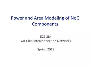
Improved NoC Router Power-Area Models technology parameters implementation parameters • interconnect parameters • device parameters • LEF/Capacitance Tables/etc. • … • Target frequency • Chip aspect ratio • Row utilization grantI reqI architectural parameters grantE reqE • # of ports; # of buffers • flit-width; # of VC • voltage, frequency Arbiter grantW reqW grantN reqN grantS reqS Request Signals Source Source Buf I Control Link Link Buf E Link Link Buf W inI outI Link Link Buf N inE outE Link Link Buf S Crossbar inW outW inN outN inS outS • Built using router layout data • Closed-form models suitable for design space exploration • Provides significant accuracy improvement compared with existing models (e.g., ORION 2.0) Write
Outline Motivation Implementation Flow and Design of Experiments Modeling Methodology Modeling Problem Power Modeling Area Modeling Experimental Results and Discussion Conclusions
Implementation Flow and Tools RTL generation from architecture Timing-driven synthesis, place and route flow Use range of architectural and implementation parameters to capture design space Nonparametric regression modeling Router RTL (Netmaker) Architectural Parameters Synthesis (Design Compiler) Implementation Parameters Power and Area Models Place + Route (SOC Encounter) Model Generation (Multiple Adaptive Regression Splines) Power / Area Reports
Design of Experiments Netmaker (Cambridge) fully synthesizable router RTL codes Libraries: TSMC (1) 130G, (2) 90GP, and (3) 65GP Tool Chain: Synopsys Design Compiler (DC), Cadence SOC Encounter (SOCE), Salford MARS 3.0 Experimental aces: Technology nodes: {130nm, 90nm, 65nm} Implementation parameters: fclk = target clock frequency ar = aspect ratio util = row utilization Architectural parameters: fw = flit-width nvc = number of virtual channels nport = number of input/output ports lbuf = buffer length (#flit buffers / VC)
Outline Motivation Implementation Flow and Design of Experiments Modeling Methodology Modeling Problem Power Modeling Area Modeling Experimental Results and Discussion Conclusions
Modeling Problem → • Accurately predict y given vector of parameters x • Difficulties: (1) which variables x to use, and (2) how different variables combine to generate y • Parametric regression: requires a functional form • Nonparametric regression: learns about the best model from the data itself For our purpose, allows decoupling of underlying architecture / implementation from modeling effort • We use nonparametric regression to model power and area of an on-chip router →
Multivariate Adaptive Regression Splines (MARS) • MARS is a nonparametric regression technique • MARS builds models of form: • Each basis function Bi(x) can be: • a constant • a “hinge” function max(0, c-x) or max(0, x-c) • a product of two or more hinge functions • Two modeling steps: • (1) forward pass: obtains model with defined maximum number of terms • (2) backward pass: improves generality by avoiding an overfit model ^ → →
Power and Area Modeling • Derive models for both dynamic and leakage power • Dynamic power is due to switching capacitance (cswitching) • Pdynamic = 0.5×α×cswitching×V2×fclk • Leakage power is due to leakage current (ileak) (subthreshold + gate) • Pleakage = ileak×V • Our modeling task: • To model dependence of (Pdynamic / α×V2×fclk)on microarchitectural and implementation parameters • To model dependence of (Pleakage / V) on microarchitectural and implementation parameters • Similarly, we model dependence of extracted area on microarchitectural and implementation parameters • Area is the sum of standard cell area
Example MARS Output Models (1) Dynamic power model of a router in 65nm technology B1 = max(0, nport - 5); B2 = max(0, 5 – nport); … B34 = max(0, fclk - 200)×B1; B35 = max(0, 200 - fclk) B1; Pdynamic = 0.5×α×(0.83 + 0.64×B1 - 0.31×B2 + 0.16×B3 … - 0.003×B33 + 0.003×B34 - 0.003×B35)×V2 Leakage power model of a router in 65nm technology B1 = max(0, nport - 5); B2 = max(0, 5 - nport); … B34 = max(0, nvc - 3)×B27; B35 = max(0, 3 - nvc)×B27; Pleakage = (0.13 + 0.04×B1 - 0.04×B2 + 0.01×B3 … - 6.59E-5×B34 - 5.53E-5×B35)×V
Example MARS Output Models (2) Area model of a router in 65nm technology B1 = max(0, nport - 5); B2 = max(0, 5 - nport); … B34 = max(0, 24 - fw)×B14; B35 = max(0, fclk - 100)×B15; Area = 0.02 + 0.01×B1 - 0.004×B2 + 0.003×B3 … - 4.59E-6×B34 - 1.23E-7×B35 Total wirelength model of a router in 65nm technology (NEW) B1 = max(0, nport - 5); B2 = max(0, 5 - nport); … B33 = max(0, 1 - ar)×B26; B34 = max(0, util - 0.7)×B8; WLtotal = 112269 + 64952.4×B1 - 31881.3×B2 … + 157.639×B33 - 321.06×B34 • Closed-form expressions with respect to architectural and implementation parameters • Suitable to drive early-stage architecture-level design exploration
Outline Motivation Implementation Flow and Design of Experiments Modeling Methodology Modeling Problem Power Modeling Area Modeling Experimental Results and Discussion Conclusions
Model Comparison (1) We compare our models against (1) models derived from parametric regression (Reg.), and (2) ORION 2.0 models We assume baseline virtual channel (VC) with FIFO buffers implemented as flip-flop registers cswitching ~ O(lbuf×fw×nport); ileak ~ O(lbuf×fw×nport×nvc) Multiplexer tree crossbar cswitching ~ O(n2port×fw); ileak ~ O(n2port×fw) VC “selection” arbitration (cf. Kumar et al. ’07) cswitching ~ O(n2port); ileak ~ O(n2port×nvc) Buffer dynamic power does not change with nvc since the number of flits arriving at each input port is the same Due to VC “selection” VC dynamic power becomes invariant to actual number of VCs Requires modeler to have knowledge about the underlying architecture / circuit implementation
Model Comparison (2) Comparison against ORION 2.0 w.r.t. microarchitectural parameters: (1) #VC (nvc), (2) flit-width (fw), (3) #port (nport), and (4) buffer length (lbuf)
Model Comparison (3) Power estimation error reductions Reg.: avg error 76.2% (24.4% 5.8%), max error 45.2% (108.4% 59.4%) ORION 2.0: avg error 82.3% (32.8% 5.8%), max error 27.4% (81.8% %59.4) Area estimation error reductions Reg.: avg error 79.4% (26.2% %5.4), max error 45.5% (111.3% 61.8%) ORION 2.0: avg error 83.8% (33.3% 5.4%), max error 28.3% (86.2% 61.8%)
Variable Importance Use MARS to identify relative variable importance using post-synthesis and post-layout data nvc and nport are dominant parameters for post-synthesis and post-layout data, respectively impact of missing layout information at post-synthesis Multiplexer crossbar power is due to (1) multiplexers and (2) interconnection grid between input / output ports With post-synthesis data interconnection data is ignored crossbar power is modeled as O(nport×log2nport) With post-layout crossbar power is modeled as O(n2port)
Model Robustness 256 different router configurations Five different scenarios to train / test our models (1) str = 1/2, (2) str = 1/3, (3) str = 1/5, (4) str = 1/10, and (5) str = 64 For (1)-(4) we train models using a fraction str of the available data points, and validate them on the rest of the data points To assess the sensitivity of the model to sample size For (5) we use 64 (out of 256) data points to train the model, and validate it across all 256 available data points To assess the generality of the model
Recent Extensions Have used same methodology to develop models for interconnect wirelength (WL) and fanout (FO) Wirelength model On average, within 3.4% of layout data 91% reduction of avg error vs. existing models (cf. Christie et al. ’00) Fanout model On average, within 0.8% of the layout data 96% reduction of avg error vs. existing models (cf. Zarkesh-Ha et al. ’00) (FO) (WL)
Outline Motivation Implementation Flow and Design of Experiments Modeling Methodology Modeling Problem Power Modeling Area Modeling Experimental Results and Discussion Conclusions
Conclusions and Future Directions Generally applicable modeling methodology that can leverage architectural parameters and RTL-to-layout implementation Achieved accurate power and area models for on-chip router Improvement over parametric regression models Power: 76.2% (45.2%) reduction of average (maximum) error Area: 79.4% (44.5%) reduction of average (maximum) error Improvement over ORION 2.0 Power: 82.3% (27.4%) reduction of average (maximum) error Area: 83.8% (28.3%) reduction of average (maximum) error Ongoing work Maximum fclk modeling w.r.t. architectural and implementation parameters Other architectural building blocks (DSP cores, DesignWare library, …) Power, performance and cost estimators for 3-D design space exploration