Download
1 / 18
210 likes | 387 Views
Advanced rate theory. Reviews in Modern Physics 62, 251-341 (1990). Advanced rate theory. Given: two states (A and C) of local stability The coordinate x describes the dynamics of the escape process. x is usually coupled to solvent coordinates. Therefore x is a stochastic variable.

E N D
Advanced rate theory Reviews in Modern Physics 62, 251-341 (1990) GK 1276
Advanced rate theory Given: two states (A and C) of local stability The coordinate x describes the dynamics of the escape process. x is usually coupled to solvent coordinates. Therefore x is a stochastic variable. GK 1276
Separation of time scales The time scale of escape clearly depends on the size of the fluctuations f(t) If we relate the fluctuations f(t) to an appropriate energy scale Enoise , transitions between the two attracting regions A and C will be infrequent whenever the condition (2.2a) Eb : energy barrier heights for forward and backward-activated processes. For systems in contact with a temperature environment at temperature T, the energy scale Enoise is given by kBT. Then, the relation reduces to (2.2b) GK 1276
Separation of time scales The time scale s describing decay within the attractor A is given by where M is the effective mass of the reacting particle. with (2.2a) and (2.2b), the time s is well separated from the time scale of escape e. In realistic systems, there will be many separate time scales s. For the discussion of the escape rate, it only matters that they are all much faster than the time scale of escape, or the inverse of the rate of escape k. GK 1276
Equation of motion for the reaction coordinate The stochastic motion of the reaction coordinate x(t) is a combined effect induced by the coupling among a multitude of environmental degrees of freedom. In principle, all these may couple directly to the reaction coordinate x(t). The dynamics of the pair is the result of a reduced description from the full phase space This approach entails new concepts, which can be loosely characterized as friction and entropy. GK 1276
Equation of motion for the reaction coordinate Entropy factor: concerns the reduction of all coupled degrees of freedom from a high-dimensional potential energy surface in full phase space to an effective potential (i.e. potential of mean force) for the reduced dynamics of the reaction coordinate. Friction: concerns the reduced action of the degrees of freedom that are lost upon contraction of the complete phase-space dynamics. Mathematics of such a reduction uses projection operators. The „coarse-grained“ dynamics can be cast either in the form of a generalized Langevin equation or in the form of a generalized master equation. GK 1276
Equation of motion for the reaction coordinate Such a reduction leads to a renormalization of mass as well as a renormalization of bare potential fields. The price to be paid for the reduction is that the resulting dynamics generally contains memory = yields a non-Markovian process (2.6a) The effect of mass renormalization is contained in a time-dependent (memory)- Friction tensor (X;t) which obeys the fluctuation-dissipation relation (2.6b) The renormalization of the bare potential occurs via the drift field (2.6c) are the corresponding stationary probabilities carrying zero flux. GK 1276
Separation of time scales For thermal systems with extremely short noise correlation times c, one can use a Markovian approximation for Eq. (2.6). Then, X(t) can be obtained from an underlying Hamiltonian dynamics in full phase space with initial coordinates and momenta distributed according to a canonical thermal equilbrium, and with the reacting particle (mass M) moving in a potential U(x) that is coupled bilinearly to a bath of harmonic oscillators. Using an infinite number of bath oscillators, Eq. (2.6) then reduces to the familiar (Markovian) Langevin equation for nonlinear Brownian motion, (2.7) Here, (t) denotes Gaussian white noise: (2.8) is a uniform, temperature-independent velocity relaxation rate. (2.7) and (2.8) are the starting point for Kramers‘ treatment of the reaction rate. GK 1276
Concepts in rate theory: 1 Flux-over-population method Farkas (1927) : evaluate steady-state current j that results if particles are continuously fed into the domain of attraction (region of x1) and subsequently are continuously removed by an observer in the neighboring domain of attraction (region of x2) beyond the transition state xb xT. This scheme results in a steady-state current with builds up a stationary nonequilibrium probability p0 inside the initial domain of attraction. Boundary conditions: (2.9) The right side of eq. (2.9) implies an absorbing boundary, where the particles are removed immediately at an infinite rate. If denotes the (nonequilibrium) population inside the initial domain of attraction, the rate of escape k is then given by This general procedure relies in practice on the explicit knowledge of a (Markovian or non-Markovian) master equation governing the time dependence for the single-event probability p(x,t) of the reaction coordinate. GK 1276
Concepts in rate theory: 2 Method of reactive flux Consider thermal systems. By noting that the (long-time) decay occurs on the same time scale e, the dynamics of spontaneous fluctuations and relaxation toward stationary equilibrium of a large non-equilibrium concentration are connected. This concept, which is valid whenever there is a clear-cut separation between time-scales, is known as „regression hypothesis“. E.g. consider the dynamics of the two relative populations na(t) and nc(t). In terms of the rate coefficients k+, k-, the population dynamic reads In equilibrium, we have in terms of the equilibrium constant K the detailed balance relation GK 1276
Method of reactive flux The relaxation of na(t) from an initial nonequilibrium deviation na(0) = na(0) – na thus reads with the relaxation rate given by The population na(t) can be described as a nonequilibrium average of a characteristic function (x) where Here, we have introduced a reaction coordinate x(q) that is positive in the domain of attraction of the metastable state A and is negative elsewhere. The expectation value denotes the equilibrium population. The fluctuations of obey where GK 1276
Method of reactive flux According to Onsager‘s regression hypothesis, the nonequilibrium average na(t) decays according to the same dynamic law as the equilibrium correlation function of the fluctuation (2.18) (2.19) This relation is not valid for short times t s. Introduce time scale obeying Let us consider the time derivative of (2.18) on this intermediate time scale . The reactive flux is given by (2.20) Thus we obtain an explicit expression for the relaxation rate (2.21) GK 1276
Equation of motion for the reaction coordinate Equivalently, we find for the forward rate (2.22) (2.21) and (2.22) hold equally well for situations in which the reaction coordinate x(t) moves primarily via spatial diffusion (strong friction) and those in which x(t) moves via inertia-dominated Brownian motion (weak friction). In the limit of eq. (2.22) for 0+, the rate can be expressed as an equilbrium average of a one-way flux at the transition state Therefore, transition-state theory always overestimates the true rate because TST ignores recrossings of reactive trajectories. GK 1276
Reactive flux Eq. (2.21) – (2.25) are analogous to the Green-Kubo formulas for transport coefficients. GK 1276
3 Mean first passage time The mean first-passage time (MFPT) is the average time that a random walker, starting from a point x0 inside the initial domain of attraction, takes to leave the domain of attraction for the first time. At weak noise, this MFPT, t(x0), becomes essentially independent of the starting point, i.e. t(x0) = tMFPT for all starting configurations away from the immediate neighborhood of the separatrix. When noting that the probability of crossing the separatrix in either direction is 0.5, the total escape time e = 2 tMFPT. Thus the rate of escape k is given by • Unfortunately, the MFPT is a rather complex notion for a general (non-Markovian) stochastic process x(t). The use of MFPT is well known for • - one-dimensional Markov processes which are of the Fokker-Planck form • - for one-dimensional master equations of the birth and death type involving nearest-neighbor transitions • - for one-dimensional master equations with one- and two-step transitions only. • … TST … variational TST … GK 1276
Kramers rate theory Kramers‘ (1940) model for a chemical reaction consists of a classical particle of mass M moving in a one-dimensional asymmetric double well potential U(x). The particle coordinate x corresponds to the reaction coordinate. All remaining degrees of freedom of reacting and solvent molecules constitute a heat bath at a temperature T, whose total effect on the reacting particle is described by a fluctuating force (t) and by a linear damping force -Mv. The resulting 2-dimensional stochastic dynamics for reaction coordinate x and the velocity v are Markovian. The time evolution of the probability density is governed by the Klein-Kramers equation GK 1276
Kramers rate theory The qualitative behavior of the nonlinear dynamic in eq. (4.4) can be easily understood. If kBT is much smaller than the expected barrier heights, the random force is acting only as a small perturbation. Its influence may typically be neglected on the time scale of the unperturbed damped deterministic motion The reaction coordinate will relax to one of the minima of the potential and the system will stay there for an extremely long time. Eventually the accumulated action of the random force will drive it over the barrier into a neighboring metastable state. GK 1276
Kramers rate theory For strong friction the reaction coordinate undergoes a creeping motion and the velocity may be eliminated adiabatically from eq. (4.1). The time evolution of the corresponding reduced probability is governed by the Smoluchowski equation Kramers required that both –U‘(x) and p(x,t) are almost constant on the thermal length scale. GK 1276