Download
1 / 26
260 likes | 268 Views
Geometry and Theory of LP. Standard (Inequality) Primal Problem: Dual Problem:. Geometry of the Prototype Example. P2. Max 3 P1 + 5 P2 s.t. P1 + < 4 (Plant 1) 2 P2 < 12 (Plant 2) 3 P1 + 2 P2 < 18 (Plant 3)

E N D
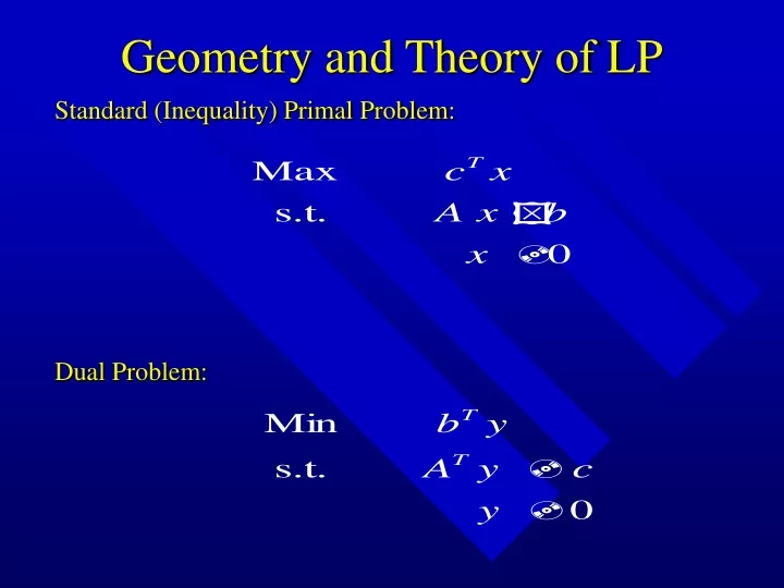
Geometry and Theory of LP Standard (Inequality) Primal Problem: Dual Problem:
Geometry of the Prototype Example P2 Max 3 P1 + 5 P2 s.t. P1 + < 4 (Plant 1) 2 P2 < 12 (Plant 2) 3 P1 + 2 P2 < 18 (Plant 3) P1, P2 > 0 (nonnegativity) Every point in this nonnegative quadrant is associated with a specific production alternative. ( point = decision = solution ) P1 0
Geometry of the Prototype Example P2 Max 3 P1 + 5 P2 s.t. P1 + < 4 (Plant 1) 2 P2 < 12 (Plant 2) 3 P1 + 2 P2 < 18 (Plant 3) P1, P2 > 0 (nonnegativity) P1 (4,0) (0,0)
Geometry of the Prototype Example P2 Max 3 P1 + 5 P2 s.t. P1 + < 4 (Plant 1) 2 P2 < 12 (Plant 2) 3 P1 + 2 P2 < 18 (Plant 3) P1, P2 > 0 (nonnegativity) (0,6) P1 (4,0) (0,0)
Geometry of the Prototype Example P2 Max 3 P1 + 5 P2 s.t. P1 + < 4 (Plant 1) 2 P2 < 12 (Plant 2) 3 P1 + 2 P2 < 18 (Plant 3) P1, P2 > 0 (nonnegativity) (0,6) (2,6) (4,3) (9,0) P1 (4,0) (0,0)
Geometry of the Prototype Example P2 Max 3 P1 + 5 P2 s.t. P1 + < 4 (Plant 1) 2 P2 < 12 (Plant 2) 3 P1 + 2 P2 < 18 (Plant 3) P1, P2 > 0 (nonnegativity) (0,6) (2,6) (4,3) (9,0) P1 (4,0) (0,0)
P2 Max 3 P1 + 5 P2 In Feasible Region (0,6) (2,6) Feasible region is the set of points (solutions) that simultaneously satisfy all the constraints. There are infinitely many feasible points (solutions). (4,3) (9,0) P1 (4,0) (0,0)
Geometry of the Prototype Example P2 Max 3 P1 + 5 P2 (0,6) (2,6) Objective function contour (iso-profit line) (4,3) (9,0) P1 (4,0) 3 P1 + 5 P2 = 12 (0,0)
Geometry of the Prototype Example 3 P1 + 5 P2 = 36 P2 Max 3 P1 + 5 P2 s.t. P1 + < 4 (Plant 1) 2 P2 < 12 (Plant 2) 3 P1 + 2 P2 < 18 (Plant 3) P1, P2 > 0 (nonnegativity) (0,6) (2,6) Optimal Solution: the solution for the simultaneous boundary equations of two active constraints (4,3) (9,0) P1 (4,0) (0,0)
Degeneracy P2 Max 3 P1 + 5 P2 s.t. P1 + < 4 (Plant 1) 2 P2 < 12 (Plant 2) 3 P1 + 2 P2 < 24 (Plant 3) P1, P2 > 0 (nonnegativity) (0,6) (2,6) The number of active constraints is more than the number of variables. (9,0) P1 (4,0) (0,0)
LP Terminology • solution (decision, point): any specification of values for all decision variables, regardless of whether it is a desirable or even allowable choice • feasible solution: a solution for which all the constraints are satisfied. • feasible region (constraint set, feasible set): the collection of all feasible solution • objective function contour (iso-profit, iso-cost line) • optimal solution (optimum): a feasible solution that has the most favorable value of the objective function • optimal (objective) value: the value of the objective function evaluated at an optimal solution • active constraint (binding constraint) • inactive constraint • redundant constraint • interior, boundary • extreme point (corner)
Unbounded or Infeasible Case • On the left, the objective function is unbounded • On the right, the feasible set is empty
Graphical Solution Seeking • Plot the feasible region. • If the region is empty, stop: the problem is infeasible; there must be conflicting constraints in the model. • Plot the objective function contour and choose the optimizing direction. • Determine whether the objective value is bounded or not. If not, stop: the problem is unbounded; there must be mistakes in model formulation. • Determine an optimal corner point. • Identify active constraints at this corner. • Solve simultaneous linear equations for the optimal solution. • Evaluate the objective function at the optimal solution to obtain the optimal value of the problem.
Theory of Linear Programming An LP problem falls in one of three cases: • Problem is infeasible: Feasible region is empty. • Problem is unbounded: Feasible region is unbounded towards the optimizing direction. • Problem is feasible and bounded: then there exists an optimal point; an optimal point is on the boundary of the feasible region; and there is always at least one optimal corner point (if the feasible region has a corner point). When the problem is feasible and bounded, • There may be a unique optimal point or multiple optima (alternative optima). • If a corner point is not “worse” than all its neighbor corners, then it is optimal.
Convexity of Feasible Region Convex Set Non-Convex Set F is a convex set if and only if for any two points, x and y, of F, their convex combination, x + (1- )y, for all real values 0 <= <= 1, is also in F.
Local Optimal => Global Optimal Convex Set Proof by contradiction: If the point is not globally optimal, then it is not locally optimal
LP Duality Standard (Inequality) Primal Problem: Dual Problem:
LP Duality (continued) Standard (Equality) Primal Form: Dual Form:
General Rules for Constructing Dual 1. The number of variables in the dual problem is equal to the number of constraints in the original (primal) problem. The number of constraints in the dual problem is equal to the number of variables in the original problem. 2. Coefficient of the objective function in the dual problem come from the right-hand side of the original problem. 3. If the original problem is amax model, the dual is aminmodel; if the original problem is amin model, the dual problem is themaxproblem. 4.The coefficient of the first constraint function for the dual problem are the coefficients of the first variable in the constraints for the original problem, and the similarly for other constraints. 5. The right-hand sides of the dual constraints come from the objective function coefficients in the original problem.
General Rules for Constructing Dual ( Continued) 6. The sense of the ith constraint in the dual is = if and only if the ith variable in the original problem is unrestricted in sign. 7. If the original problem is man (min ) model, then after applying Rule 6, assign to the remaining constraints in the dual a sense the same as (opposite to ) the corresponding variables in the original problem. 8. The ith variable in the dual is unrestricted in sigh if and only if the ith constraint in the original problem is an equality. 9. If the original problem is max (min) model, then after applying Rule 8, assign to the remaining variables in the dual a sense opposite to (the same as) the corresponding constraints in the original problem. Max model Min modelxi >= 0 <=> ith constraint>= xi <= 0 <=> ith constraint <= xi free <=> ith constraint = ith const <= <=> yi >= 0 ith const >= <=> yi <= 0 ith const = <=> yi free
Economic Interpretation 1.Max Model: the shadow price for the ith constraint = the optimal value of the ith variable in the dual. 2. Min Model: the shadow price for the ith constraint = - the optimal value of the ith variable in the dual. 3. Suppose Factory 1’s production problem is Max 3x1 + 5x2 s.t. x1 <= 4 2x2 <= 12 3x1 + 2x2 <= 18 x1, x2 >= 0 Suppose that the management of Factory 2 decides to BUY the raw material in factory 1. What are ‘fair price’ for the three raw material? Amount Factory 2 pays = 4y1 + 12y2 + 18y3 Of course, Factory 2 wants to pay as less as possible. Its goal is to Min 4y1 + 12y2 + 18y3
Economic Interpretation ( continued ): However, the prices must satisfy Factory 1 such that Factory 1 is willing to sell. Factory 1 sees that if it has 1 unit raw material 1 and 3 units of raw material 3, it could produce on unit product 1 for a profit $3. Thus, to satisfy Factory 1, Factory 2 will cover the loss of product 1 in Factory 1 due to the sell: y1 + 3y3 >= 3 The same is true for Product 2 in Factory 1: 2y2 + 2y3 >=5 Finally, Factory 2 faces the optimal pricing problem min 4y1 + 12 y2 + 18y3 s.t. y1 + 3y3 >= 3 2y2 + 2y3 >= 5 y1, y2, y3 >= 0 It provides ‘fair prices’ in the sense of prices that yield the minimum acceptable liquidation payment.
Relations between Primal and Dual 1. The dual of the dual problem is again the primal problem. 2. Either of the two problems has an optimal solution if and only if the other does; if one problem is feasible but unbounded, then the other is infeasible; if one is infeasible, then the other is either infeasible or feasible/unbounded. 3. Weak Duality Theorem: The objective function value of the primal (dual) to be maximized evaluated at any primal (dual) feasible solution cannot exceed the dual (primal) objective function value evaluated at a dual (primal) feasible solution. cTx >= bTy (in the standard equality form)
Relations between Primal and Dual (continued) 4. Strong Duality Theorem: When there is an optimal solution, the optimal objective value of the primal is the same as the optimal objective value of the dual. cTx* = bTy* 5. Complementary Slackness Theorem:Consider an inequality constraint in any LP problem. If that constraint is inactive for an optimal solution to the problem, the corresponding dual variable will be zero in any optimal solution to the dual of that problem. x*j (c-ATy*)j = 0, j=1,…,n.
Optimality Conditions Primal Feasibility: Dual Feasibility: Strong Duality: or Complementary Slackness: