Download
1 / 104
1.05k likes | 1.64k Views
THE NCEP CLIMATE FORECAST SYSTEM REANALYSIS. THE ENVIRONMENTAL MODELING CENTER NCEP/NWS/NOAA. The NCEP Climate Forecast System Reanalysis

E N D
THE NCEP CLIMATE FORECAST SYSTEM REANALYSIS THE ENVIRONMENTAL MODELING CENTER NCEP/NWS/NOAA
The NCEP Climate Forecast System Reanalysis Suranjana Saha, Shrinivas Moorthi, Hua-Lu Pan, Xingren Wu, Jiande Wang, Sudhir Nadiga, Patrick Tripp, Robert Kistler, John Woollen, David Behringer, Haixia Liu, Diane Stokes, Robert Grumbine, George Gayno, Jun Wang, Yu-Tai Hou, Hui-ya Chuang, Hann-Ming H. Juang, Joe Sela, Mark Iredell, Russ Treadon, Daryl Kleist, Paul Van Delst, Dennis Keyser, John Derber, Michael Ek, Jesse Meng, Helin Wei, Rongqian Yang, Stephen Lord, Huug van den Dool, Arun Kumar, Wanqiu Wang, Craig Long, Muthuvel Chelliah, Yan Xue, Boyin Huang, Jae-Kyung Schemm, Wesley Ebisuzaki, Roger Lin, Pingping Xie, Mingyue Chen, Shuntai Zhou, Wayne Higgins, Cheng-Zhi Zou, Quanhua Liu, Yong Chen, Yong Han, Lidia Cucurull, Richard W. Reynolds, Glenn Rutledge, Mitch Goldberg Bulletin of the American Meteorological Society Volume 91, Issue 8, pp 1015-1057. doi: 10.1175/2010BAMS3001.1
WHAT IS AN ANALYSIS SYSTEM? • WHAT IS A REANALYSIS SYSTEM ?
0Z OBS 6Z OBS 12Z OBS DA DA DA MG MG MG 0Z ANL 6Z ANL 12Z ANL ONE DAY OF ANALYSIS OBS: Observations DA: Data Assimilation MG: Model Guess ANL: Analysis
Analysis is always ongoing in operational weather prediction centers in real time • Consecutive analyses over many years may constitute some sort of a climate record • Analysis also provide initial states for model forecasts
What is a Reanalysis ? • analysis made after the fact (not ongoing in real time) • with an unchanging model to generate the model guess (MG) • with an unchanging data assimilation method (DA) • no data cut-off windows and therefore more quality controlled observations (usually after a lot of data mining)
Motivation to make a Reanalysis ? • To create a homogeneous and consistent climate record Examples: R1/CDAS1: NCEP/NCAR Reanalysis (1948-present) Kalnay et al., Kistler et al R2/CDAS2 : NCEP/DOE Reanalysis (1979-present) Kanamitsu et al ERA40, ERA-Interim, MERRA, JRA25, NARR, etc…. • To create a large set of initial states for Reforecasts (hindcasts, retrospective forecasts..) to calibrate real time extended range predictions (error bias correction).
An upgrade to the NCEP Climate Forecast System (CFS) is being planned for 18 Jan 2011. For a new Climate Forecast System (CFS) implementation Two essential components: A new Reanalysis of the atmosphere, ocean, seaice and land over the 32-year period (1979-2010) is required to provide consistent initial conditions for: A complete Reforecast of the new CFS over the 29-year period (1982-2010), in order to provide stable calibration and skill estimates of the new system, for operational seasonal prediction at NCEP
For a new CFS implementation (contd) • Analysis Systems : Operational GDAS: Atmospheric (GADAS)-GSI Ocean-ice (GODAS) and Land (GLDAS) 2. Atmospheric Model : Operational GFS New Noah Land Model 3. Ocean Model : New MOM4 Ocean Model New Sea Ice Model
An upgrade to the coupled atmosphere-ocean-seaice-land NCEP Climate Forecast System (CFS) is being planned for 18 Jan 2011. This upgrade involves changes to all components of the CFS, namely: • improvements to the data assimilation of the atmosphere with the new NCEP Gridded Statistical Interpolation Scheme (GSI) and major improvements to the physics and dynamics of operational NCEP Global Forecast System (GFS) • improvements to the data assimilation of the ocean and ice with the NCEP Global Ocean Data Assimilation System, (GODAS) and a new GFDL MOM4 Ocean Model • improvements to the data assimilation of the land with the NCEP Global Land Data Assimilation System, (GLDAS) and a new NCEP Noah Landmodel
For a new CFS implementation (contd) • An atmosphere at high horizontal resolution (spectral T382, ~38 km) and high vertical resolution (64 sigma-pressure hybrid levels) • An interactive ocean with 40 levels in the vertical, to a depth of 4737 m, and horizontal resolution of 0.25 degree at the tropics, tapering to a global resolution of 0.5 degree northwards and southwards of 10N and 10S respectively • An interactive 3 layer sea-ice model • An interactive land model with 4 soil levels
There are three main differences with the earlier two NCEP Global Reanalysis efforts: • Much higher horizontal and vertical resolution (T382L64) of the atmosphere (earlier efforts were made with T62L28 resolution) • The guess forecast was generated from a coupled atmosphere – ocean – seaice - land system • Radiance measurements from the historical satellites were assimilated in this Reanalysis To conduct a Reanalysis with the atmosphere, ocean, seaice and land coupled to each other was a novelty, and will hopefully address important issues, such as the correlations between sea surface temperatures and precipitation in the global tropics, etc.
6 Simultaneous Streams 1 Dec 1978 to 31 Dec 1986 1 Nov 1985 to 31 Dec 1989 1 Jan 1989 to 31 Dec 1994 1 Jan 1994 to 31 Mar 1999 1 Apr 1998 to 31 Mar 2005 1 Apr 2004 to 31 Dec 2009 Full 1-year overlap between streams to account for ocean, stratospheric and land spin up issues Reanalysis covers 31 years (1979-2009) + 5 overlap years And will continue into the future in real time.
ONE DAY OF REANALYSIS 12Z GSI 18Z GSI 0Z GSI 6Z GSI 0Z GLDAS 12Z GODAS 18Z GODAS 0Z GODAS 6Z GODAS 9-hr coupled T382L64 forecast guess(GFS + MOM4 + Noah) 1 Jan 0Z 2 Jan 0 Z 3 Jan 0Z 4 Jan 0Z 5 Jan 0Z 5-day T126L64 coupled forecast ( GFS + MOM4 + Noah )
ONE DAY OF REANALYSIS • Atmospheric T382L64 (GSI) Analysis at 0,6,12 and 18Z, using radiance data from satellites, as well as all conventional data • Ocean and Sea Ice Analysis (GODAS) at 0,6,12 and 18Z • From each of the 4 cycles, a 9-hour coupled guess forecast (GFS at T382L64) is made with 30-minute coupling to the ocean (MOM4 at 1/4o equatorial, 1/2o global) • Land (GLDAS) Analysis using observed precipitation with Noah Land Model at 0Z • Coupled 5-day forecast from every 0Z initial condition was made with the T126L64 GFS for sanity check.
R1 Troposphere CFSR Troposphere 28 levels 64 levels R1 Stratosphere CFSR Stratosphere Courtesy: Shrinivas Moorthi The vertical structure of model levels as a meridional cross section at 90E
The linear trends are 0.66, 1.02 and 0.94K per 31 years for R1, CFSR and GHCN_CAMS respectively. (Keep in mind that straight lines may not be perfectly portraying climate change trends). Courtesy: Huug van den Dool
5-day T126L64 forecast anomaly correlations Courtesy: Bob Kistler
Response of Prec. To SST increase : warming too quick in R1 and R2 SST-Precipitation Relationship in CFSR Precipitation-SST lag correlation in tropical Western Pacific simultaneous positive correlation in R1 and R2 Courtesy: Jiande Wang
CFSR data dump volumes, 1978-2009, in GB/month Courtesy: Jack Woollen
Performance of 500mb radiosonde temperature observations The top panel shows monthly RMS and mean fits of quality controlled observations to the first guess (blue) and the analysis (green). The fits of all observations, including those rejected by the QC, are shown in red. The bottom panel shows the 00z data counts of all observations (in red) and those which passed QC and were assimilated in green. Courtesy: Jack Woollen
Another innovative feature of the CFSR GSI is the use of the historical concentrations of carbon dioxide when the historical TOVS instruments were retrofit into the CRTM. Courtesy: http://gaw.kishou.go.jp
Tropical Cyclone Processing • The first global reanalysis to assimilate historical tropical storm information was the JRA-25 reanalysis (Onogi, et.al. 2007). It assimilated synthetic wind profiles (Fiorino, 2002) surrounding the historical storm locations of Newman, 1999. • A unique feature of the CFSR is its approach to the analysis of historical tropical storm locations. The CFSR applied the NCEP tropical storm relocation package (Liu et. al., 1999), a key component of the operational GFS analysis and prediction of tropical storms. • By relocating a tropical storm vortex to its observed location prior to the assimilation of storm circulation observations, distortion of the circulation by the mismatch of guess and observed locations is avoided. • Fiorino (personal communication) provided the CFSR with the historical set of storm reports (provided to NCEP by the National Hurricane Center and the US Navy Joint Typhoon Warning Center) converted into the operational format. • A measure of the ability of the assimilation system to depict observed tropical storms is to quantify whether or not a reported storm is detected in the guess forecast. A noticeable improvement starts in 2000 coincident with the full utilization of the ATOVS satellite instruments, such that between 90-95% of reported tropical storms are detected.
Transition to Real Time CFSR • The operational GSI had gone through several upgrades during the CFSR execution. In March 2009 a major addition was made to the CRTM to simulate the hyper-spectral channels of the IASI instrument, onboard the new ESA METOP satellite and NOAA-19 was added in Dec 2009. • In order to continue to meet the goal of providing the best available initial conditions to the CFS, in the absence of staff and resources to maintain the CFSR GSI into the future, it was decided to make the transition to the CDAS mode of CFSR in April 2008. • The operational GSI, present and future implementations, will replace the CFSR GSI, and the coupled prediction model will be “frozen” to that of the CFS v2. • Historical observational datasets would be replaced with the operational data dumps.
The global number of temperature observations assimilated per month by the ocean component of the CFSR as a function of depth for the years 1980-2009. Courtesy: Dave Behringer
The global distribution of all temperature profiles assimilated by the ocean component of the CFSR for the year 1985. The distribution is dominated by XBT profiles collected along shipping routes. Courtesy: Dave Behringer
The global distribution of all temperature profiles assimilated by the ocean component of the CFSR for the year 2008. The Argo array (blue) provides a nearly uniform global distribution of temperature profiles Courtesy: Dave Behringer
The subsurface temperature mean for an equatorial cross-section Courtesy: Sudhir Nadiga
The Diurnal Cycle of SST in CFSR The diurnal cycle of SST in the TAO data (black line) and CFSR (blue line) in the Equatorial Pacific for DJF (top three panels) and JJA (bottom three panels). T 165E 165E 110W 170W 110W DJF 170W DJF JJA JJA Courtesy: Sudhir Nadiga
The vertically averaged temperature (surface to 300 m depth) for CFSR for 1979-2008, and its difference with observations from World Ocean Atlas Courtesy: Sudhir Nadiga
Zonal and meridional surface velocities for CFSR (top left and top right) and differences between CFSR and drifters from the Surface Velocity Program of TOGA (bottom panels). Courtesy: Sudhir Nadiga
The first two EOFs of the SSH variability for the CFSR (left) and for TOPEX satellite altimeter data (right) for the period: 1993-2008. The time series amplitude factors are plotted in the bottom panel. Courtesy: Sudhir Nadiga
Monthly mean sea ice concentration for the Arctic from CFSR (6-hr forecasts) Courtesy: Xingren Wu
Monthly mean Sea ice extent (106 km2) for the Arctic (top) and Antarctic (bottom) from CFSR (6-hr forecasts). 5-year running mean is added to detect long term trends. Courtesy: Xingren Wu
Problem for Sea-Ice Concentration in CFSRR for 2009: Due to the degradation of one of the DMSP F15 sensor channels in February, and a problem from F13 in early May 2009
Extent of Sea-Ice for 2009 (from R. Grumbine) Mid Feb – f15 ‘bad’ Early May – f13 problem Mar 5 – drop of f15 May 13 – Addition of amsre May 2009 Sea-Ice in CFSRR
Possible Solution: (1) Model guess (2) Persistence (3) … May 2009 Sea-Ice in CFSRR