Download

1 / 60
610 likes | 1.04k Views
Image Enhancement and Filtering Techniques. EE4H, M.Sc 0407191 Computer Vision Dr. Mike Spann m.spann@bham.ac.uk http://www.eee.bham.ac.uk/spannm. Introduction . Images may suffer from the following degradations:

E N D
Image Enhancement and Filtering Techniques EE4H, M.Sc 0407191 Computer Vision Dr. Mike Spann m.spann@bham.ac.uk http://www.eee.bham.ac.uk/spannm
Introduction • Images may suffer from the following degradations: • Poor contrast due to poor illumination or finite sensitivity of the imaging device • Electronic sensor noise or atmospheric disturbances leading to broad band noise • Aliasing effects due to inadequate sampling • Finite aperture effects or motion leading to spatial
Introduction • We will consider simple algorithms for image enhancement based on lookup tables • Contrast enhancement • We will also consider simple linear filtering algorithms • Noise removal
Histogram equalisation • In an image of low contrast, the image has grey levels concentrated in a narrow band • Define the grey level histogram of an image h(i) where : • h(i)=number of pixels with grey level= i • For a low contrast image, the histogram will be concentrated in a narrow band • The full greylevel dynamic range is not used
Histogram equalisation • Can use a sigmoid lookup to map input to output grey levels • A sigmoid function g(i) controls the mapping from input to output pixel • Can easily be implemented in hardware for maximum efficiency
Histogram equalisation • θcontrols the position of maximum slope • λ controls the slope • Problem - we need to determine the optimum sigmoid parameters and for each image • Abetter method would be to determine the best mapping function from the image data
Histogram equalisation • A general histogram stretching algorithm is defined in terms of a transormation g(i) • We require a transformation g(i) such that from any histogram h(i) :
Histogram equalisation • Constraints (N x N x 8 bit image) • No ‘crossover’ in grey levels after transformation
Histogram equalisation • An adaptive histogram equalisation algorithm can be defined in terms of the ‘cumulative histogram’ H(i) :
Histogram equalisation • Since the required h(i) is flat, the required H(i) is a ramp: h(i) H(i)
Histogram equalisation • Let the actual histogram and cumulative histogram be h(i) and H(i) • Let the desired histogram and desired cumulative histogram be h’(i) and H’(i) • Let the transformation be g(i)
Histogram equalisation • Since g(i) is an ‘ordered’ transformation
Histogram equalisation • Worked example, 32 x 32 bit image with grey levels quantised to 3 bits
0 197 197 1.351 - 1 256 453 3.103 197 2 212 665 4.555 - 3 164 829 5.676 256 4 82 911 6.236 - 5 62 993 6.657 212 6 31 1004 6.867 246 7 20 1024 7.07 113 Histogram equalisation
Histogram equalisation • ImageJ demonstration • http://rsb.info.nih.gov/ij/signed-applet
Image Filtering • Simple image operators can be classified as 'pointwise' or 'neighbourhood' (filtering) operators • Histogram equalisation is a pointwise operation • More general filtering operations use neighbourhoods of pixels
Image Filtering • The output g(x,y) can be a linear or non-linear function of the set of input pixel grey levels {f(x-M,y-M)…f(x+M,y+M}.
Image Filtering • Examples of filters:
Linear filtering and convolution • Example • 3x3 arithmetic mean of an input image (ignoring floating point byte rounding)
Linear filtering and convolution • Convolution involves ‘overlap – multiply – add’ with ‘convolution mask’
Linear filtering and convolution • We can define the convolution operator mathematically • Defines a 2D convolution of an image f(x,y) with a filter h(x,y)
Linear filtering and convolution • Example – convolution with a Gaussian filter kernel • σdetermines the width of the filter and hence the amount of smoothing
Linear filtering and convolution Noisy Original Filtered σ=3.0 Filtered σ=1.5
Linear filtering and convolution • ImageJ demonstration • http://rsb.info.nih.gov/ij/signed-applet
Linear filtering and convolution • We can also convolution to be a frequency domain operation • Based on the discrete Fourier transform F(u,v) of the image f(x,y)
Linear filtering and convolution • The inverse DFT is defined by
Linear filtering and convolution • F(u,v) is the frequency content of the image at spatial frequency position(u,v) • Smooth regions of the image contribute low frequency components to F(u,v) • Abrupt transitions in grey level (lines and edges) contribute high frequency components toF(u,v)
Linear filtering and convolution • We can compute the DFT directly using the formula • An N point DFT would require N2 floating point multiplications per output point • Since there are N2 output points , the computational complexity of the DFT is N4 • N4=4x10⁹ for N=256 • Bad news! Many hours on a workstation
Linear filtering and convolution • The FFT algorithm was developed in the 60’s for seismic exploration • Reduced the DFT complexity to 2N2log2N • 2N2log2N~106 for N=256 • A few seconds on a workstation
Linear filtering and convolution • The ‘filtering’ interpretation of convolution can be understood in terms of the convolution theorem • The convolution of an image f(x,y) with a filter h(x,y) is defined as:
Linear filtering and convolution • Note that the filter mask is shifted and inverted prior to the ‘overlap multiply and add’ stage of the convolution • Define the DFT’s of f(x,y),h(x,y), and g(x,y) as F(u,v),H(u,v) and G(u,v) • The convolution theorem states simply that :
Linear filtering and convolution • As an example, suppose h(x,y) corresponds to a linear filter with frequency response defined as follows: • Removes low frequency components of the image
Linear filtering and convolution DFT IDFT
Linear filtering and convolution • Frequency domain implementation of convolution • Image f(x,y)N x N pixels • Filter h(x,y) M x M filter mask points • Usually M<<N • In this case the filter mask is 'zero-padded' out to N x N • The output image g(x,y) is of size N+M-1 x N+M-1 pixels. The filter mask ‘wraps around’ truncating g(x,y) to an N x N image
Linear filtering and convolution • We can evaluate the computational complexity of implementing convolution in the spatial and spatial frequency domains • N x Nimage is to be convolved with an M x Mfilter • Spatial domain convolution requires M 2 floating point multiplications per output point or N 2 M 2 in total • Frequency domain implementation requires 3x(2N 2 log 2N) +N 2 floating point multiplications ( 2 DFTs + 1 IDFT + N 2multiplications of the DFTs)
Linear filtering and convolution • Example 1, N=512, M=7 • Spatial domain implementation requires 1.3 x 10⁷ floating point multiplications • Frequency domain implementation requires 1.4 x 10⁷ floating point multiplications • Example 2, N=512, M=32 • Spatial domain implementation requires 2.7 x 10⁸ floating point multiplications • Frequency domain implementation requires1.4 x 107floating point multiplications
Linear filtering and convolution • For smaller mask sizes, spatial and frequency domain implementations have about the same computational complexity • However, we can speed up frequency domain interpretations by tessellating the image into sub-blocks and filtering these independently • Not quite that simple – we need to overlap the filtered sub-blocks to remove blocking artefacts • Overlap and add algorithm