Download
1 / 75
850 likes | 1.21k Views
Chapter 6 Frequency Response & Systems Concepts. AC circuit analysis methods to study the frequency response of electrical circuits Understanding of frequency response aided by the concepts of phasors and impedance. Filtering – a new concept will be explored. Objectives.

E N D
Chapter 6 Frequency Response & Systems Concepts • AC circuit analysis methods to study the frequency response of electrical circuits • Understanding of frequency response aided by the concepts of phasors and impedance. • Filtering – a new concept will be explored Këpuska 2005
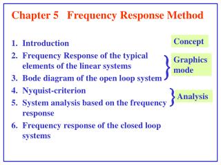
Objectives • Understand significance of frequency domain analysis • Introduction of Fourier series as a tool for computation of Fourier spectrum. • Analyze first and second-order electrical filters by determining their filtering properties. • Computation of frequency response and its graphical representation as Bode plot. Këpuska 2005
Sinusoidal Frequency Response • Provides a circuit response to a sinusoidal input of arbitrary frequency. • The frequency response of a circuit is a measure of voltage or current (magnitude and phase) as a function of the frequency of excitation (source) signal. Këpuska 2005
Methods to Compute Frequency Response • Thevenin equivalent source circuit: + Zs Z1 ZT VL ~ ~ VT VT Z2 - Këpuska 2005
Load Voltage VT ZT ZL ~ VT Këpuska 2005
Frequency Response • From definition: • VL(j) is a phase-shifted and amplitude-scaled version of VS(j) ⇨ Këpuska 2005
Frequency Response (cont) • Phasor form of the load voltage: Këpuska 2005
Example 6.1 • Compute the frequency response Hv(j) of the circuit for R1= 1k, C=10F; and RL= 10k. Këpuska 2005
Magnitude & Phaze Këpuska 2005
Fourier Analysis • Let x(t) be a periodic signal with period T. • x(t) = x(t+nT) for n=1,2,3,… Këpuska 2005
Fourier Series • A signal x(t) can be expressed as an infinite summation of sinusoidal components know as Fourier Series: • Sine-cosine (quadrature) representation • Magnitude and Phase form: • Fundamental Frequency and Period T: Këpuska 2005
Fourier Series • It can be shown • Or similarly Këpuska 2005
Fourier Series Aproximation • Infinite summation practically not possible • Replaced by finite summation that leads to approximation. • Higher order coefficients; n, are associated with higher frequencies; (2/T)n. ⇒ • Better approximations require larger bandwidths. Këpuska 2005
Odd and Even Functions Fourier Series Këpuska 2005
Frequency Spectrum Këpuska 2005
Computation of Fourier Series Coefficients Këpuska 2005
Example of Fourier Series Approximation • Square wave and its representation by a Fourier series. (a) Square wave (even function); (b) first three terms; (c) sum of first three terms Këpuska 2005
Example 6.3 Computation of Fourier Series Coefficients • Problem: Compute the complete Fourier Spectrum of the sawtooth function shown in the Figure below for T=1 and A=1: Këpuska 2005
Solution • x(t) is an odd function. • Evaluate the integral in equation Këpuska 2005
Solution (cont) • Spectrum computation: Këpuska 2005
Matlab Simulation • Components of the sawtooth wave function: Këpuska 2005
Matlab Simulation • Fourier Series approximation of sawtooth wave function Këpuska 2005
Example 6.4 • Problem: Compute the complete Fourier series expansion of the pulse waveform shown in the Figure for /T=0.2 • Plot the spectrum of the signal Këpuska 2005
Solution • Expression for x(t) • Evaluate Integral Equations: Këpuska 2005
Solution (cont) Këpuska 2005
Spectrum Computation • Magnitude: • Phase: Këpuska 2005
Graphical Representation Këpuska 2005
Matlab Simulation Këpuska 2005
Matlab Simulation Këpuska 2005
Linear Systems Response to Periodic Inputs • Any periodic signal x(t) can be represented as a sum of finite number of pure periodic terms: Këpuska 2005
General Input-Output Representation of a System Këpuska 2005
Linear Systems • For Linear Systems - by definition Principle of superposition applies: T{ax1(t) + bx2(t)} = aT{x1(t)} + bT{x2(t)} a x1 ax1[n] + bx2[n] T{} y= T{ax1(t) + bx2(t)} x2 b a aT{x1[n]} T{} x1 y= aT{x1(n)}+bT{x2(n)} T{} x2 bT{x2[n]} b Këpuska 2005
Linear System View of a Circuit • Output of a circuit y(t) as a function of the input x(t): Këpuska 2005
Example 6.6 Response of Linear System to Periodic Input • Problem: • Linear system: • Input: sawtooth waveform approximated with only first two Fourier components of the input waveform. Këpuska 2005
Solution • Approximation of the sawtooth function with first two terms of Fourier Series: • Spectrum Computation: Këpuska 2005
Frequency Response • Magnitude and Phase • Computation of Frequency Response for two frequency values of 1 = 8 and 2 = 16: Këpuska 2005
Frequency Response (cont) • Computation of steady-state periodic output of the system: Këpuska 2005
Matlab Simulation Këpuska 2005
Matlab Simulation Këpuska 2005
Filters • Low-Pass Filters Simple RC Filter Këpuska 2005
Low-Pass Filter Këpuska 2005
Low-Pass Filter • =0 • H(j)=1 ⇨ Vo(j)=Vi(j) • >0 Këpuska 2005
Low-Pass Filter Cutoff Frequency Këpuska 2005
Example 6.7 • Compute the response of the RC filter to sinusoidal inputs at the frequencies of 60 and 10,000 Hz. • R=1k, C=0.47F, vi(t)=5cos(t) V • 0=1/RC=2,128 rad/sec • = 120 rad/sec ⇒ /0 = 0.177 • = 20,000 rad/sec ⇒ /0 = 29.5 Këpuska 2005
Solution Këpuska 2005
High-Pass Filters Këpuska 2005
High-Pass Filter • The expression in previous slide can be written in magnitude-and-phase form: Këpuska 2005
High-Pass Filter Response Këpuska 2005
Band-Pass Filters Këpuska 2005
Frequency Response of Band-Pass Filter Këpuska 2005