Download
1 / 25
330 likes | 771 Views
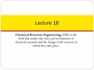
Lecture 16 Final Version. Contents. Combinations of Solutions: Solid Bodies in a Potential Flow (Rankine Oval etc.) Cylinder in Uniform Flow Cylinder with Circulation in a Uniform Flow Pressure Distribution Around the Cylinder Kutta-Joukowski Lift Theorem

E N D
Lecture 16Final Version Contents Combinations of Solutions: Solid Bodies in a Potential Flow (Rankine Oval etc.) Cylinder in Uniform Flow Cylinder with Circulation in a Uniform Flow Pressure Distribution Around the Cylinder Kutta-Joukowski Lift Theorem Circulation and Lift for Aerofoil Applications
Instructions now on www as PDF file. (Instructions should also appear as hardcopies via your pigeon hole • Deadline for submission extended until Friday Week 12 (= Fri. 19 Jan. 2007) • Submission sheet will appear on www soon-ish (and also via pigeon holes) Design Project
COMBINATIONS OF SOLUTIONS: SOLID BODIES IN A POTENTIAL FLOW • Recall: Can use PRINCIPLE OF SUPERPOSITION for velocity potential. • In addition, have shown that for incompressible, irrotational flow, stream function also satisfies Laplace Eq. So can similarly construct flow solutions by combining S.F. associated with uniform flow, source/sink flow and line-vortex flow. • In fact, we will almost exclusively use stream function here because we are interested in pattern of streamlines; once we find stream function, we can use fact that it is constant along streamlines to plot out streamlines. Uniform Flow and Source: THE RANKINE BODY What happens if we combine... ? (1) Cartesian Coordinates: (2) Polar Coordinates: • (1)/(2) represent complete descriptions of flow field. But what does it look like?... • To graph lines of constant , first look for STAGNATION POINTS. There ... Thus, both velocity components must be zero… Differentiate to get expressions for velocity components ...
Cartesian Coordinates: Continued... (3) (4) • For v=0 Eq. (4) requires ... ...with this Eq. (3) gives... STAGNATION POINT at • Polar Coordinates: and Since m, r positive choose... to get a solution for STAGNATION POINT at
In both cases same location for Stagnation Point ... Continued... Cartesian Coordinates Polar Coordinates We repeated ourselves to demonstrate that either coordinate system can be used. In general choose the one that makes the analysis easiest. • Now use for distance between origin and stagnation point: • Find S.L. that arrives at stagnation point and divides there. Using ... along this S.L., use a known point - the stagnation point - to evaluate constant. With Eq (2) from above ... where suffix s denotes ‘along particular streamline through stagnation point’. • Streamline found by equatingEq (2) to the constant and rearranging... (5)
Plotting stagnation streamline: Continued... • Stagnation streamline defines shape of (imaginary) solid half-body which may be fitted inside streamline boundary; remember flow does not cross streamline … or solid boundary. Call this special S.L. SURFACE STREAMLINE. • Body shape named after Scottish engineer W.J.M. Rankine (1820-1872). • Now only have stagnation/surface. To get other S.L.’s, choose point, determine constant for S.L. through point and then sketch particular S.L. through this point by compiling a table as above.
How Does Flow Speed Vary Along Surface Streamline? • Recall velocity components in cartesian coord. from Eqs. (3)/(4) : Continued... • Flow speed is: NOW RECALL: (6) • To find flow speed on body surface, VS , evaluate Eq. (6) subject to (5) for surface streamline. This gives ...
Note: Since we know surface flow speed, we can evaluate static pressure at any point on surface. Using Bernoulli equation along central streamline that divides into surface streamline and, as usual, ignoring gravitational term... Continued... Hence we get the non-dimensional pressure coefficient :
Uniform Flow and Sink (instead of Source) Continued... Stream Function Sink Source (previous case) Cart. Coord. Pol. Coord. • Only difference: plus sign(s) changed into minus sign(s)! Hence, for sink expect a very similar analysis as above for source. Source Sink S.P. • Note: In real world (inviscid) flow pattern for sink would not be observed! Flow would initially follow body contour but (due to viscosity) detach at separation points indicated by S.P. in sketch for sink. The phenomenon of SEPARATION will be covered later. At this stage learn that... Potential flows do NOT model ALL features of a real flow!!!This has lead to potential flow often being termed IDEAL FLOW.
Uniform Flow + Source + Sink Obvious question now is what happens for ... We consider ‘symmetric’ case where: Strength Location Source Sink We cannot have both at origin now! What would happen if both at origin? • By considering the two sketches on previous slide we can anticipate shape of surface streamline and resulting body... … an oval. • Using superposition, can readily write stream function for this flow: (1) • Second and third terms can be combined using: To give a more concise form for stream function
From either of the two forms of S.F. on previous slide, one can determine velocity components Continued... (2) (3) • Now find stagnation points, where u=v=0. From Eq. (3) one sees that when y=0 then v=0. • Substitute y=0 into Eq. (2) and then find value of x which gives that u=0. • After some manipulation the solutions for x are: • Hence, stagnation points at: and • Now determine value of S.F. for surface streamline from Eq (1). (1) - repeated It can be seen that this is trivial and that
Rankine Oval then looks like ... Continued... • We already determined value of L. Can find points of maximum velocity and minimum pressure at shoulders +/-h, of oval using similar methods. All these parameters are a function of the... … basic dimensionless parameter In summary one obtains • As one increases dimensionless parameter d from zero to large values, oval shape increases in size and thickness from flat plate of length 2c to huge, nearly circular ‘cylinder’. Here think of increase when • All Rankine ovals, except very thin ones, have large adverse pressure gradient on leeward surface. Thus, boundary-layer will separate in rear, broad wake flow develops, inviscid pattern unrealistic in that region.
Overall Strategy for Plotting Streamlines from Stream Function was... Write down stream function for flow by appropriately combining individual solutions for source, sink and line vortex as a sum: Note: Huge choice as far as selction of parameters is concerned! Souce strength, vortex direction of rotation, strength … ... Calculate expressions for vel. components u, v from Determine coord.of stagnation point(s) via u=0 , v =0. Determine value of stream function passing through (stagnation) point by substituting coordinates of (stagnation) point(s) into the stream function. Set stream function equal to the value you have determined for point in question. Determine values of x, y (or r, ) that satisfy this expression and plot to obtain streamline. Choose new point x,y
Cylinder in a Uniform Flow From previous it should be obvious how one can find stream function for a cylinder (circle) in a uniform flow ... • Turn Rankine oval into circle by allowing ... • Achieved by moving source and sink closer to origin ... Limit (c=0) would ultimately ‘cancel’ pair! • Ensure their influence remains by allowing m to increase in size. Necessary limit is... with • Recall that Rankine oval had S.F. ... • Now then the argument of tan-1 goes to zero... • Noting that gives • DefineDOUBLET STRENGTH: Stream Function for Cylinder Flow (1) Note: Merging of source and sink as above produces structure known as DOUBLET.
More convenient to work in polar coordinates! S.F. can be written ... Continued... (1) • From Eq. (1) can get velocitycomponents in usual way...
(2) Wherewe used... Continued... (3) • CHECK that this flow really does represent a cylinder in uniform flow. Stagnation points: Eq. (3) : • Substitute these angles into Eq.(2) Hence,... Stagnation points: • Surface S.L. VALUE by substituting one stag. point into Eq. (1)... • Now get equation for Surface S.L. by equating Eq. (1) to zero ... As required surface S.L. is circle with radius
Continued... Uniform Flow + Doublet = Flow over a Cylinder • Velocity Componentson cylinder surface are obtained, by setting r=R, from... Eq. (2) Eq. (3) Might have expected to find that radial flow component is zero on surface - flow cannot pass through (solid) cylinder wall! • Note also that maximum flow speed occurs at where it is respectively. Means in both cases (top and bottom half of cyl.) flow is from left to right! On top negative value as velocity points in clockwise (negative angle) direction. On bottom in anti-clockwise (positive angle) direction. • Finally, note symmetry of flow about both the x- and y- axes. What does this tell you about the pressure distribution on the cylinder surface… remember the Bernoulli Equation!
Since we can now mathematically describe … Continued... ...we can, in principle, also describe flow through an arbitrary array of cylinders as, for instance, the flow shown in the photo below. We simply need to put several doublets in our uniform flow.
Without performing calculation, can see in preceding flow no net lift or drag on cylinder since pressure distribution on surface symmetric about x- and y-axis.. Cylinder with Circulation in a Uniform Flow • In order to generate lift need to break symmetry. Achieved by introducing line vortex of strength, K, at origin which introduces circulation . • Note that this does not violate the flow around cylinder: line vortex produces a component of velocity only. Hence, we are still adhering to condition that flow cannot pass through cylinder boundary. • Working from S.F. for cylinder in uniform flow additional inclusion of line vortex gives: (1) Use result that radius of resulting cylinder is : And set : (1) Velocity Components
So, on surface (r=R), velocity components are: Continued... • Surface Stagnation points also need: Note: By setting vortex strength zero (K=0), recover flow over cylinder in uniform flow with stagnation points at • Plotting,… Choose value for K,… Now first get value of S.F. for r=R,... then set S.F. equal to that value,… then compile table r vs. angle… This gives particular streamline through stagnation points. Then choose any other point in flow field not on stagnation streamline,… determine value of S.F. for this point,… set S.F. equal to that value,… then compile table r vs. angle… This gives streamline through the chosen particular points… Then choose another point in flow field… etc (compare flow chart from beginning of lecture). For various values of K the following, flow fields emerge...
Continued... • Can now also describe flow through an arbitrary array of cylinders when each of them is rotating! (Note: In photo below cylinders are not rotating)
To evaluate press. on cyl. surface use Bernoulli Eq. along S.L. that originates far upstream where flow is undisturbed. Ignoring grav. forces: Pressure Distribution Around the Cylinder • Re-arranging... • Substituting for flow speed gives... … difference in pressures between surface and undisturbed free stream (1) In particular for non-rotating cylinder where K=0: (2) Def.: Pressure Coefficient Only top half of cyl. shown.
Qualitative behaviour of Continued... for various values of . • Best way of interpreting above graphs is to think of flow velocity and radius being constant while vortex strength is increasing from one plot to next. • When plotting graphs I did not explicitly specify velocity or radius! I simply used different numeric values for in order to illustrate behaviour of graph. I have not considered if any of these cases may not be realizable in reality or not!.
Equation (1) … … can be used to calculate net lift and drag acting on cylinder! Continued... Sketch (A) Sketch (B) • In Sketch (b) ... • Hence, integration around cylinder surface yields total L and D ... where b is width (into paper) of cylinder. Substituting for pressure using Eq. (1), and integrating (most terms drop out), leads to following results: Or, lift per unit width: Thus, drag zero… a remarkable result!
Net lift is indicated in sketch below. ... Note that if a line vortex is used which rotates in mathematically positive sense (anti-clockwise) then resulting lift is negative, i.e. downwards. Continued... • Final notes:How is lift generated? ... From sketch above and from pressure profiles plotted earlier it is evident how this is physically achieved… Breaking of the flow symmetry in x-axis means that flow round lower part of cylinder is faster than round top - this means that pressure is lower round bottom and so a net downward force results. Notice that symmetry in y-axis is retained … symmetry of pressure on left-hand and right-hand faces is retained and so there is no net drag force. Keep in mind that our analysis was for an ideal fluid (i.e. there is no viscosity). In a real flow would fore-aft symmetry be retained? • Lastly, since lift is proportional to circulation, we wish to make circulation large to generate a large lifting force. In applications of above flow this is achieved by spinning cylinder to produce large vorticity… but is there a limit to how much circulation we should produce?