Download
1 / 98
980 likes | 1.25k Views
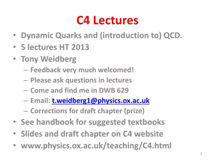
C4 Lectures. Dynamic Quarks and (introduction to) QCD. 5 lectures HT 2013 Tony Weidberg Feedback very much welcomed! Please ask questions in lectures Come and find me in DWB 629 Email: t.weidberg1@physics.ox.ac.uk Corrections for draft chapter (prize) See handbook for suggested textbooks

E N D
C4 Lectures • Dynamic Quarks and (introduction to) QCD. • 5 lectures HT 2013 • Tony Weidberg • Feedback very much welcomed! • Please ask questions in lectures • Come and find me in DWB 629 • Email: t.weidberg1@physics.ox.ac.uk • Corrections for draft chapter (prize) • See handbook for suggested textbooks • Slides and draft chapter on C4 website • www.physics.ox.ac.uk/teaching/C4.html
Outline • Review of evidence for quarks from static quark model. • How to study particle structure • Review of Rutherford scattering and how to measure size of nucleus (form factors). • Scattering off nucleons in nuclei • Simple Quark Parton Model • ve scattering • nq scattering • np scattering • ep and mp scattering • Predictions of the QPM direct evidence for spin ½ fractionally charged partons quarks are real! • Gluons and extension to QCD • Scaling violations gluon distribution • Hadron – hadron interactions. 2 2 2 2 2 2
Static Quark Model • SU(3) and quark multiplets • Allowed understanding of bizarre number of “elementary particles”. • SU(3) badly broken so predictions approximate. • Charmonimum and bbar States • Spectra strikingly similar to positronium • Can we get more direct evidence for quarks? • Yes we can with DIS These lectures! 3 3 3 3 3 3
Rutherford Scattering (1) • Alpha –gold scattering; prototype for all scattering experiments. • Use Fermi Golden Rule • H’ is Coulomb interaction • Plane waves for initial and final states 4 4 4 4 4 4
Rutherford Scattering (2) • Matrix element • Sub for V(r) and define momentum transfer • Use spherical polar r axis // q q.r=qr cos(θ) 5 5 5 5 5 5
Rutherford Scattering (3) • Integral is divergent (cf classical result) • Modify potential by factor exp(-r/a) and let a∞ • Let a∞ gives matrix element 6 6 6 6 6 6
Rutherford Scattering (4) • Density of states • Cross section and transition rates: T=s F and flux F=v. • Ignore nuclear recoil: • Gives Rutherford scattering cross section 7 7 7 7 7 7
Form Factor (1) • Rutherford scattering cross section doesn’t depend on any fixed scale in problem. • We had assumed point like nucleus. • What happens for finite sized nuclei? • Coulomb potential modified: • Matrix element modified 8 8 8 8 8 8
Form Factor (2) • Matrix element modified compared to pure Coulomb by form factor • Form factor is Fourier transform of charge distribution in 3D space to momentum space. • In principle: measure deviations from pure Coulomb potential F(q2) inverse FT gives ρ(r). • Why doesn’t this work in practice? 9 9 9 9 9 9
Form Factor (3) • Requires probe with λ<<R ie qR>>1 (high energy!). • Assume toy model for charge distribution ie • Gives form factor (work it out yourself!) • q << m F(q2) ~ constant because resolution too poor. • q >> m F(q2) ~ 1/q4 and σ suppressed by 1/q8 10 10 10 10 10 10
Form Factor (4) • Real example! Data and fit to charge distribution. • 153 MeV e- scattering on Au • Large difference between data and point nucleus. • Fits to two models for charge distribution. 11 11 11 11 11 11
Approximatefit to uniformchargedistribution (sharp edge) Good fit to realistic charge distribution 12 12 12 12 12 12
Summary so far … • Low energy scattering shows • Scaling cross section evidence for point like nucleus (within resolution l= h/p) • Higher energy scattering shows • Fixed scale in cross section evidence for finite size nucleus • Scattering data form factors charge distribution in nucleus 13 13 13 13 13 13
Nucleon Scattering (1) • Next steps into the nucleus … lets look for evidence of nucleons inside the nucleus from scattering experiments … • Conservation of 4 momentum and energy 14 14 14 14 14
Nucleon Scattering (2) • Recoil invariant mass W and 4-momtum transfer • Elastic scattering off entire nucleus W=M 15 15 15 15 15 15
Nucleon Scattering (3) e- He scattering fixed angle 450, Ee=400 MeV Sharp peak: elastic scattering off nucleussmeared peak: elastic scattering off p (Fermi motion) What do we expect with partons inside proton? 16 16 16 16 16
Quark-Parton Model • Assume QPM is correct predictions for DIS compare with data. (0) Kinematics for DIS (1) (2) (3) Generalise to n quarks (4) Generalise to n nucleon (5) Extend to e/m nucleon (6) Compare with data! 17 17 17 17 17
Kinematics (1) • Assume quarks have mass m=xM • Elastic scattering off quark: Define Q2=-q2 nb only need scattered electron measurement 18 18 18 18 18
Kinematics (2) • x can also represent fractional proton momentum carried by quark. • DIS large Q2 neglect quark mass compared to energy evaluate quark mass after scattering. • x can represent either mass fraction or momentum fraction (infinite momentum frame) p.q LI use lab frame 19 19 19 19 19
Kinematics (3) • Relation between CMS angle and lab energies. • LT from CMS to lab (b=1) for scattered and initial lepton. Define y=n/E (0<y<1) CMS scattering angle q* = 0 for incident lepton Elastic E=E’ 20 20 20 20 20
Anti-neutrino e scattering (1) • Consider W contribution • W couples to LH e- and RH anti n • high energy chirality = helicity. • Very simple spin structure • Amplitude from projecting m=1/2 to m’=1/2 21 21 21 21 21
(Anti) Neutrino e scattering (2) • Cross section proportional to |A|2 • Phase space proportional to p2=s/4. • GF Fermi coupling constant • Numerical factors requires Feynman rules 22 22 22 22 22
Neutrino e scattering • Jz=0 so J=0 or J=1 not as simple … • Crossing symmetry: anti-particles & amplitudes • Matrix element for crossed diagrams same with p_incoming - p_outgoing. • Compare ne and ne p1<->p3 • Isotropic, phase space + GF + numerical factor 3 ne q* 1 2 e- e- 4 23 23 23 23 23
Neutrino Quark Scattering (1) • Universality of CC weak interactions. • In nq scattering: • Now write down cross sections for (anti) neutrino on (anti) quark scattering by analogy with (anti) neutrino scattering on e- 24 24 24 24
Neutrino quark scattering q and q’ not same (CKM). Also ignore threshold effects 25 25 25 25
Neutrino Nucleon Scattering • QPM: scattering of leptons from nucleon is incoherent sum of scattering off quarks • Assumption only valid for large q2>>1 GeV2 • Justification from QCD and experiment • Let q(x) be the pdf for finding quark with momentum fraction x in a proton. • What does q(x) mean? • QPM can’t predict q(x) need fits to data. • Many clear predictions can be checked with data 26 26 26 26
Neutrino Nucleon Scattering (1) • Combine all ingredients cross section for measurable quantities! 27 27 27 27
Neutrino Detector • High energy beam nm. • What final state particles do we want to detect? • Detector shape and size ? • Passive material? • Active material? • Readout?
Neutrino Nucleon Scattering (2) • Compare y distributions with data • If anti-quarks negligible: • nN : flat y anti-n N: (1-y)2 • Data fits combination of flat and (1-y)2 quarks are spin ½ and interact by a parity violating interactions. 29 29 29 29
Neutrino Nucleon Scattering (3) Integrate in x and y to get total cross sections. Assume quarks dominant y integrals trivial x integral ~ unity Neutrino larger than anti-neutrino See next slide for data Cross sections scale like s quarks are point like If quarks had finite size form factor suppression. 30 30 30 30
Neutrino Nucleon Scattering (4) S=2mE s/E constant vs E Quarks are point like! 31 31 31
Parton Distribution Functions (1) • How to determine the PDFs qi(x) from data? • Rewrite QPM prediction to allow fits to data. • Compare with formula allowed by Lorentz Invariance 32 32 32
Parton Distribution Functions (2) • Fit F2 and F3 to data q and anti-q • Which quarks are we considering? • Assume nucleons only contain u,d,s and anti-quarks 33 33 33
Parton Distribution Functions (3) • Which quarks do n see ? 34 34 34
Parton Distribution Functions (4) • What about neutrons? • Assume SU(2) symmetry: 35 35 35
Nuclear Targets What about nuclei? Assume isoscalar target I=0 Just average n and p and assume s=sbar 36 36 36
Sum Rules (1) • Important consistency checks of QPM • Divide q(x) into valence and sea • 2 valence u + 1 valence d in proton Gross-Llewellyn-Smith sum rule • Check with data 37 37 37
GLS Sum Rule • Agrees with data at large Q2 • Disagreement at low Q2 can be explained by higher order QCD corrections. 38 38 38
Addler Sum Rule • Addler Sum Rule: • Two valence u and one valence d SA=1 • 2SA=2.02 ± 0.4 (D. Allasia, et al., Z. Phys. C 28 (1985) 321.) • Agrees with data! 39 39 39
Momentum Sum • Integrate F2 momentum fraction carried by quarks • Naïve expectiation: I=1 but I=0.44 at Q2=10 GeV2. • ~ ½ momentum is carried by particles that don’t experience weak force • First evidence for gluons! • More direct evidence when we look at QCD. 40 40 40
Charged Lepton Probes • Advantages of e/m • Higher intensity beams • ep (HERRA) access to larger range in x and q2. • Disadvantages? • How to calculate the lepton – nucleon s? • Calculate e m scattering • Generalise to e q scattering • Generalise to eN scattering (QPM) 41 41 41
em Scattering (1) • Work by analogy with elastic ne scattering • EM interactions, photon massless and strength given by a. • Need to evaluate spin factor F 42 42 42
em Scattering (2) • Spin factor F • Calculate amplitude for each spin configuration • Sum over final spin states • Average over initial spin states • For (1) and (2): JZ=0 same angular distribution as ne isotropic. • For (3) : JZ=1 same rotation matrices as for 43 43 43
em Scattering (3) • For (4): JZ=-1 rotation matrices gives • Averaging over initial spins and summing over final spin states • EM parity conserving equal amplitudes for LH and RH (high energy –ive and +ive H) 44 44 44
Elastic e Quark Scattering • Fractional charge of quark flavour i, is qi • Momentum fraction x cms energy squared of e quark: 45 45
e/m Nucleon DIS • Same assumptions as for n DIS: • Incoherent scattering off individual quarks • Momentum distribution functions fi(x) • cf general phenomenological formula 46 46
Quark Spin (1) • Equating powers y QPM and phenomenological formula (Callan-Gross) • Data agrees with spin ½ and excludes spin 0. • Simple explanation? • Quark spin also measured in e+e- 2 jets. /2 47 47
Quark Spin (2) • e+e- qq 2 jets • Assume jet direction = quark • Helicity conservation for EM interaction • Coupling is LR and LR • Jz=+1 or Jz=-1 • Rotation matrix for J=1, m=1 ,m’=1 and m=-1,m’=-1 amplitude
Quark Spin (3) • Data from e+e- annihilation at Petra • Agrees with 1+cos2q • Confirms quark spin=1/2.
Scaling • Most critcial prediction of QPM is scaling SF depend on x but not Q2 at high Q2 and n. • Data show approximate scaling. • If quarks had finite size very large form factor suppression. • Slow (log) variations with Q2 can be explained by QCD. • Quarks are point like within resolution of current experiments 50 50